Dashboard & Data Explorer: Guide for Users and Developers

1 Introduction

1.1 Overview

The Dashboard & Data Explorer (to be publicly available online) is a specialised analytical tool designed to monitor and visualise the financial execution of Portugal’s Official Development Assistance (ODA) and Strategic Cooperation Programmes.
Among its many features, it offers a comprehensive overview of ODA financial flows to priority partner countries (beneficiaries): Angola, Cabo Verde, Guinea-Bissau, Mozambique, São Tomé and Príncipe, and Timor-Leste.

1.2 Purpose

The primary goal of this application is to facilitate transparency and analytical insights regarding Portuguese cooperation. It allows users to:
- Track financial execution (e.g., against indicative budgets defined in Memorandums of Understanding signed between Portugal (donor) and the partner country).
- Analyse sectoral distribution of aid (e.g., Health, Education).
- Explore geographical distribution of projects.
- Drill down into specific projects and funding entities, etc..

Target Audience
This dashboard is intended for:
- Policy Makers and Strategists: To assess the progress of cooperation programmes.
- Analysts and Researchers: To explore detailed financial flows and sectoral allocations.
- General/Specialised Public: To access transparent information regarding Portuguese development cooperation.

1.3 Open Source Alignment

The European Commission encourages the transformative, innovative, and collaborative potential of open source. This dashboard aligns with the European Commission Open Source Software Strategy ¹ by:

¹ The European Commission has launched a call for evidence on the upcoming Open Digital Ecosystem Strategy which will set out:
- a strategic approach to the open source sector in the EU that addresses the importance of open source as a crucial contribution to EU technological sovereignty, security and competitiveness
- a strategic and operational framework to strengthen the use, development and reuse of open digital assets within the Commission, building on the results achieved under the 2020-2023 Commission Open Source Software Strategy.

Leveraging Open Technologies: The solution is built entirely on open-source technologies (R, Shiny, Docker), ensuring no licensing costs for the institution.
Avoiding Vendor Lock-in: By relying on community-driven standards rather than proprietary platforms, the project eliminates dependency on specific vendors.
Promoting Transparency: The use of open-source code fosters trust and allows for public scrutiny and collaboration, essential values in development cooperation.

2 Dashboard & Data Explorer: Guide for Users

This guide will help user navigate the interface, use the available filters, and interpret the various visualisations.
The application is organised into tabs, typically representing different modules (e.g., ODA Analysis). The layout generally consists of a Global Sidebar Filters on the left for controls and a Display Area on the right for results.

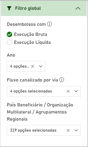
2.1 Using Global Sidebar Filters (Filtro global)

The (collapsible) sidebar controls determine what data is shown across the entire page.

2.1.1 Execution Type

for Users

Choose between:
- Execução Bruta (to inspect Gross ODA flows): Total amounts disbursed.
- Execução Líquida (to inspect Net ODA flows): Total amounts disbursed (gross) minus amounts received (reimbursements) - relevant for financial instruments like loans.
Note: If reimbursements (repayments) exceed disbursements, Net ODA will be negative.

for Developers

Ensure server-side filters respect the brutaliquida input and that any aggregation uses sum(SomaDeAPD, na.rm = TRUE) consistently to avoid NAs affecting Net calculations.

2.1.2 Time Period

for Users

Use the Ano (Year) selector to filter the data.
- Select a specific year to see annual execution.
- Select “Todos” (All) to view the cumulative execution over the available time period.

for Developers

When implementing the year filter, coerce inputs to numeric (as.numeric(input$year)) only when not equal to “Todos” to prevent parsing errors.

2.1.3 Bilateral / Multilateral ODA channels

for Users

This filter allows user to distinguish between different aid delivery channels:

Bilateral: Aid provided directly from Portugal to a partner country.
Multilateral: Contributions made to international organisations (e.g., United Nations, World Bank), which then distribute the aid.
Todos (All): View both channels combined.

Selecting a channel here will dynamically update the options available in the “Beneficiary Country / Multilateral Organization” filter.

2.1.4 Beneficiary Country / Multilateral Organization

for Users

This dropdown menu changes based on user selection in the “Bilateral / Multilateral” filter:

If Bilateral is selected: The list will show all beneficiary countries receiving contributions from Portugal. User can select one or more countries to analyse.
If Multilateral is selected: The list will show international organisations to which Portugal contributes.
Functionality: The dropdown supports searching, allowing user to quickly find a specific country or organisation.

for Developers

Populate the recipient dropdown dynamically based on the channel selection and consider using shinyWidgets::virtualSelectInput for large lists to improve performance.

2.2 Using Display Area

2.2.1 Temporal Trends (Evolução)

Line and bar timeline charts show the evolution of financial execution over time. These are useful for identifying trends in ODA financial flows.

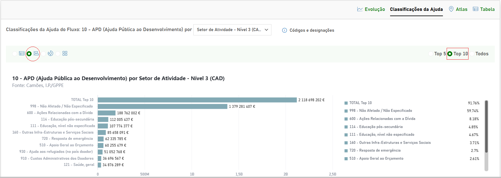
2.2.2 Summary tables for the major ODA trends (Clasificações da Ajuda)

The dashboard uses summary tables to present the major ODA trends.

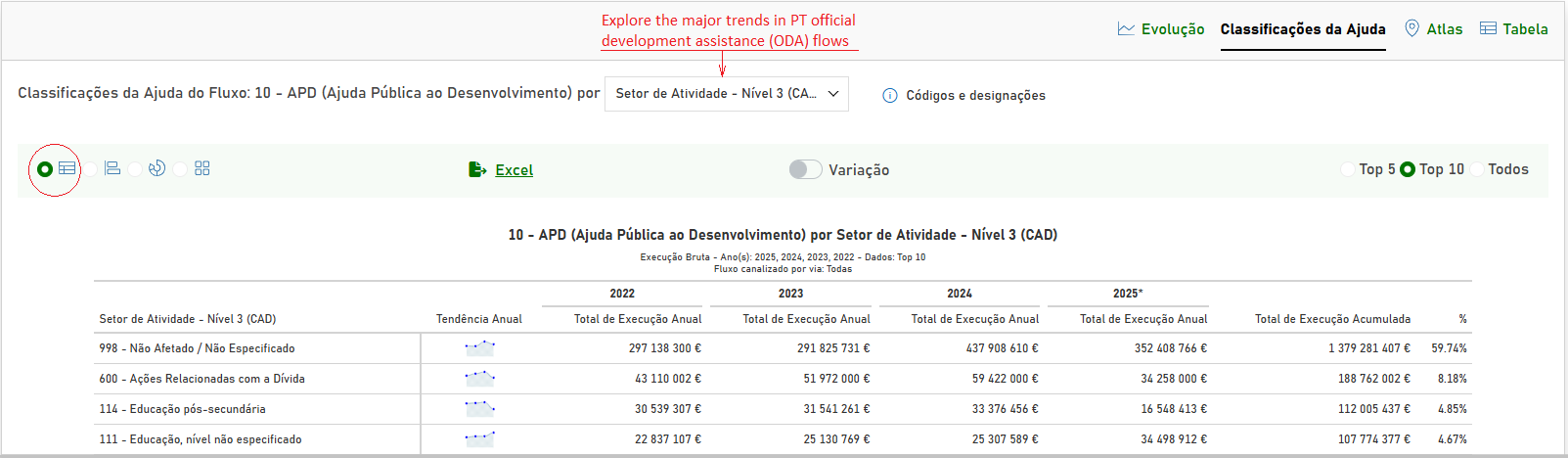
Summary tables across the major ODA trends

for Users

Hierarchical View: Data is often grouped (e.g., by Sectors or Markers). Click the arrow icons to expand or collapse these groups.
Summary tables: Small line charts illustrate how financial execution changes over time, serving as helpful visual indicators for spotting trends in financial flows.
Distributional charts: Bar, donuts and treemap display how funds are allocated across the major ODA trends. Hover over different categories to see the exact value.

for Developers

Ensure hierarchical gt tables preserve ordering and indentation when exported to Excel (see get_excel_js_helpers for conventions used by the JS exporter). Implemented in R/helpers/excel_js_helpers.R and referenced in R/modules/mod_apd.R and R/modules/mod_pec.R.

2.2.3 Interactive Map (Atlas)

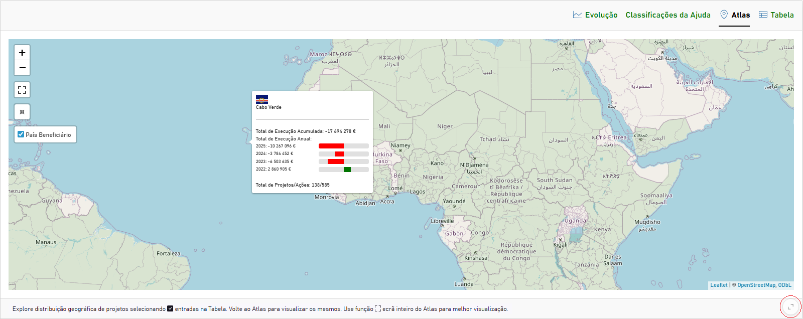
The map visualises the geographical distribution of financial execution over time.

for Users

Popups: Hover over a coloured country shape to view:
- Total Execution: The total amount for the selected period.
- Trend: A detailed bar chart showing the year-over-year evolution. Green bars indicate positive flows; red bars indicate negative flows.

for Developers

When building popups, normalize widths using the local maximum absolute value per country to ensure negative bars render correctly, see calculate_shapes_apd_geo2 function - implemented in R/helpers/apd_helpers.R and referenced in R/modules/mod_apd.R.

2.2.4 Searchable Interactive Table (Tabela)

The dashboard uses searchable interactive table to present detailed financial data.

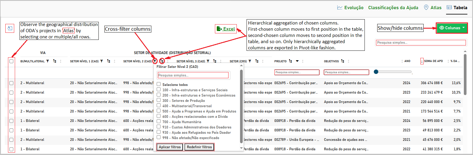
for Users

Use column filters to narrow down projects before exporting.
- Hierarchical Aggregation View: Data can be grouped. Click the arrow icons to expand or collapse these groups.
- Filtering: User can cross-filter specific columns using the text boxes or dropdowns in the table headers.

for Developers

Implement both client-side and server-side filtering support. For large tables prefer client-side reactable JS filters for UX and use server-side filtering for export endpoints.

2.2.5 Exporting Data

for Users

Users can download data for their own analysis.

Excel Export: Look for the Excel icon button (usually green) near data tables.
- Clicking this will generate an .xlsx file containing the data currently visible in the table.
- Note: A progress bar overlaid on the specific button while the file is being generated.
Chart Export: Some charts have a toolbar (usually at the top right) that allows user to download the visualisation as a SVG, PNG or CSV file or user can often right-click a chart to save it as an image.

2.3 Troubleshooting

for Users

Loading Times: Large datasets may take a moment to load. Please watch for the loading dots.
Missing Data: If a chart or table is empty, ensure that filter selection corresponds to a period where active projects existed.

3 Technical Documentation: Guide for Developers

3.1 Design Summary

3.1.1 Application Structure

The application employs a modularised Shiny architecture designed for maintainability and scalability. It follows principles of separation of concerns (SoC) by organizing code into specific directories. For example, UI and Server module logic reside in R/modules/, functional helpers in R/helpers/, and static assets in www/. The app.R launcher uses dynamic sourcing to ensure new components are registered automatically.

for Users

This project is modular to support reusability; users can request new reports by specifying required filters and visual outputs without touching module wiring.

for Developers

Follow the R/modules and R/helpers separation: keep side-effect free functions in helpers and UI/server wiring in modules. Use source_files() in app.R for dynamic loading.

File Organisation: the following diagram illustrates the high-level refactored structure of 📂directories and 📜files.

📂dashboard_bslib/
├── 📂css/
│   └── 📜custom.css
├── 📂data/
│   ├── 📜dadosAPD.parquet
│   ├── 📜dadosAPDBruta.parquet
│   └── 📜pec_apd_bruta.parquet
├── 📂js/
│   ├── 📜excel-export.js
│   ├── 📜export_excel_gt.js
│   └── 📜export_excel_reactable.js
├── 📂json/
│   ├── 📜apd_geo2.parquet
│   └── 📜palop_tl.parquet
├── 📂R/
│   ├── 📂helpers/
│   │   ├── 📜apd_helpers.R
│   │   ├── 📜data_loader.R
│   │   ├── 📜excel_js_helpers.R
│   │   ├── 📜panel_data.R
│   │   ├── 📜panel_helpers.R
│   │   ├── 📜reactable_js_helpers.R
│   │   └── 📜utils.R
│   ├── 📂modules/
│   │   ├── 📜mod_apd.R
│   │   ├── 📜mod_info.R
│   │   └── 📜mod_pec.R
│   ├── 📜app_server.R        # Application-wide server logic
│   ├── 📜app_ui.R            # Top-level UI and navigation
│   ├── 📜global.R            # Global variables and memory sharing
│   └── 📜utils_helpers.R     # Shared data aggregation logic
├── 📂www/
│   ├── 📜ao.svg
│   └── 📜... flags, image content
└── 📜app.R

Root Directory summary (key items and responsibilities):

app.R: Minimal entry point that sources R/helpers/ and R/modules/, and launches the Shiny app.
R/:
- app_server.R & app_ui.R: Define the main server logic and user interface structure, integrating the various modules.
- global.R: Used for global constants and configuration loaded at startup.
- R/modules/: Each file is a self-contained Shiny module (e.g., mod_pec.R, mod_info.R) and encapsulates the UI and Server logic for a specific section of the dashboard (keeps reactive logic here).
- R/helpers/: Contains utility functions separated by domain (small pure-R helpers, JS snippets, static choice lists):
  - apd_helpers.R: Data processing logic for APD/ODA.
  - data_loader.R:
  - excel_js_helpers.R:
  - reactable_js_helpers.R: JavaScript bindings for custom UI interactions.
  - utils.R: General utility functions (e.g., file sourcing, common formatting, naming conventions) used across modules.
- R/app_ui.R, R/app_server.R: App-level UI and server wiring; set up themes, global reactives and dependency injection for data services.
data/: Stores the primary datasets in Parquet format for efficient reading (e.g., dadosAPD.parquet, pec_apd_bruta.parquet). Prefer lazy reads via arrow::open_dataset() and SQL via DuckDB when extracting distinct values.
Styling and Scripts: Additional assets for client behaviour and styling
- css/: Custom CSS stylesheets (e.g., custom.css) for UI customisation.
- js/: Custom JavaScript files (e.g., excel-export.js) for extending Shiny functionality.
Assets:
- www/: Static web assets like images, icons (ao.svg, flags) served by Shiny.
- json/: Geo-spatial data files (e.g., apd_geo2.parquet, palop_tl.parquet) used for mapping. Read with sfarrow::st_read_parquet().

Developer notes and conventions:

Sourcing: use R/helpers/utils.R > source_files() from app.R so adding a new helper/module requires no edits to app.R.
Namespacing: UI functions should call ns <- NS(id); server code should use session$ns when DOM IDs are needed for JS selectors.
Large static objects (choices, DetailsList items, channel lists) should live in R/helpers/ to keep modules focused on reactive logic.
Background work: heavy filtering and parquet scanning should be run via shiny::ExtendedTask (mirai) or DuckDB/arrow-backed queries; avoid full dplyr::collect() before filtering.
Exports & canonical names: keep a single source-of-truth for constants (e.g., apd_entidade_static_groups implemented in R/helpers/apd_helpers.R and referenced in R/modules/mod_apd.R) and import/reference it from modules rather than duplicating definitions.

This structure aims to make the codebase easy to navigate for contributors: modules focus on reactive wiring and UI, helpers on pure logic and JS snippets, and data assets remain clearly separated for reproduction and testing.

3.1.1.1 Architecture Diagram

The following diagram conceptually illustrates the high-level file structure and the relationships between the main entry point, modules, and data sources.

graph TD
    subgraph Root
        App[app.R]
        Global[global.R]
    end

    subgraph Helpers[R/helpers/]
        Utils[utils.R]
        APD_Helpers[apd_helpers.R]
        JS_Helpers[_js_helpers.R]
    end

    subgraph Modules[R/modules/]
        ModPEC[mod_pec.R]
        ModAPD[mod_apd.R]
        ModInfo[mod_info.R]
    end

    subgraph Data[data/]
        ParquetFiles[(Parquet Files)]
    end

    subgraph Legend
        direction LR
        LegScript[R Script]
        LegData[(Data Source)]
        LegSolid[Source] -->|Direct Call| LegTarget1[Target]
        LegDotted[Source] -.->|Lazy Load| LegTarget2[Target]
    end

    App --> Global
    App --> Utils
    App --> APD_Helpers
    App --> JS_Helpers
    App --> ModPEC
    App --> ModAPD
    App --> ModInfo
    
    ModPEC -.-> ParquetFiles
    ModAPD -.-> ParquetFiles

3.1.1.2 Key Components

Entry Point app.R:
Instead of a monolithic code structures, app.R is minimal. It uses a helper function source_files() to dynamically load all scripts from the R/helpers and R/modules directories, ensuring that new components are automatically registered without modifying the launcher.

source_files() helper:
Implemented in R/helpers/utils.R and referenced in app.R.
This utility function iterates through a specified directory and sources all .R files found within it. This pattern simplifies development by removing the need to manually add a source() call for every new helper or module file created.
Deployment Configuration:
The Dockerfile defines a multi-stage build that restores R packages using {renv}, copies the application code and assets, and configures the Shiny Server.

3.1.1.3 Dependency Injection

The application implements a Dependency Injection (DI) pattern to manage external dependencies such as data repositories and configuration settings.
- Decoupling: Services (e.g., data loaders) are instantiated at the application root and passed to modules as arguments, rather than being hardcoded within the modules.
- Testability: This architecture allows for the injection of mock objects during testing, isolating module logic from external data sources.

Example Implementation:

# In R/app_server.R
# 1. Define the service (dependency)
data_service <- list(
  get_data = function() { arrow::open_dataset("data/pec_apd_bruta.parquet") }
)

# 2. Inject into the module server
mod_pec_server("pec_analysis", data_service = data_service)

# In the Module (R/modules/mod_pec.R)
mod_pec_server <- function(id, data_service) {
  moduleServer(id, function(input, output, session) {
    # 3. Use the injected service
    data <- reactive({
      data_service$get_data() |> dplyr::collect()
    })
  })
}

3.1.2 User Interface (UI) and User Experience (UX)

3.1.2.1 Modern and Structured UI

The {bslib} package creates a clean, professional, and well-organised UI layout based on Bootstrap (an open-source front-end framework that web developers use to build mobile-friendly sites and applications. It provides a collection of pre-designed templates, CSS styles, and JavaScript components to help developers efficiently and effectively create visually appealing and consistent web interfaces). The Bootswatch free theme “pulse” (one of many free themes for Bootstrap) gives a contemporary feel with a distinct colour palette and modern typography.

Key structural elements include:
- Sidebar Layout: bslib::layout_sidebar() provides a responsive structure where filters reside in a collapsible sidebar, maximizing space for data visualization.
- Accordions: bslib::accordion() organizes complex filter groups into collapsible panels, reducing visual clutter.
- Tabbed Navigation: bslib::navset_card_underline() allows users to switch seamlessly between different views (Map, Summary, Charts, Data Table) within the same context, maintaining focus.

for Users

The dashboard structure is consistent across all modules, making it easier to learn and use different sections of the application.

for Developers

Leverage bslib’s layout utilities (layout_sidebar, accordion) to maintain a clean and responsive interface that adapts to different screen sizes.

3.1.2.2 Rich Interactive Components

The application leverages several packages to enhance standard Shiny inputs and provide a richer user experience.

1. Efficient Selection with shinyWidgets::virtualSelectInput

Standard select inputs can be slow when rendering thousands of options. virtualSelectInput uses virtualization to render only the visible options, significantly improving performance for large lists like “PEC” or “Ano”.

# In R/modules/mod_pec.R (UI)
shinyWidgets::virtualSelectInput(
  inputId = ns("pec"),
  choices = NULL, # Dynamically updated
  label = "PEC",
  multiple = FALSE,
  search = FALSE,
  placeholder = "Selecione PEC",
  searchPlaceholderText = "Pesquise...ou selecione todos",
  width = "270px",
  keepAlwaysOpen = TRUE
)

2. Enhanced Radio Buttons with shinyWidgets::prettyRadioButtons

These provide a more modern look compared to default radio buttons, with support for icons and animations.

# In R/modules/mod_pec.R (UI)
shinyWidgets::prettyRadioButtons(
  inputId = ns("pecbrutaliquida"),
  label = " ",
  choices = "Execução Bruta",
  selected = "Execução Bruta",
  thick = TRUE,
  icon = icon("check"),
  plain = TRUE,
  status = "primary",
  animation = "rotate"
  # prettyRadioButtons uses native <input type="radio">, which handles role="radio" and aria-checked automatically.
)

3. Microsoft Fluent UI Components with shiny.fluent

Developer can use {shiny.fluent} for professional UI elements like MessageBar for context/warnings and ActionButton for specific interactions.

# Example: MessageBar for data context
# In R/modules/mod_pec.R (UI)
shiny.fluent::MessageBar(
  span("Dados relativos aos PECs (ano de 2025) são preliminares..."),
  isMultiline = FALSE,
  truncated = TRUE,
  messageBarType = 1, # Warning type
  messageBarIconProps = list("iconName" = "Warning")
)

4. Modern Icons with phosphoricons

The {phosphoricons} provides a consistent and clean icon set used in navigation panels.

# In R/app_ui.R
bslib::nav_panel(
  title = list(
    phosphoricons::ph(
      name = "textbox",
      weight = "thin",
      fill = "steelblue",
      title = "Programa"
    ),
    "Programa"
  ),
  # ... content ...
)

3.1.2.3 User Feedback

The application prioritizes user feedback to ensure responsiveness and clarity during operations.

1. Loading Screens with waiter

{waiter} is used to show a loading screen or spinner while the application or specific outputs are initialising.

2. Progress Bars with waitress

For long-running operations like Excel exports, waitress provides a progress bar overlaid on the specific button or element triggering the action.

# UI: Initialize Waitress
# In R/modules/mod_pec.R (UI)
waiter::useWaitress(color = "#007400")

# Server: Create Waitress instance linked to a button
# In R/modules/mod_pec.R (Server)
waitress_pec <- waiter::Waitress$new(
  selector = paste0("#", ns("export_pec")),
  theme = "overlay",
  infinite = TRUE
)

# Server: Start and Stop
shiny::observeEvent(input$export_pec, {
  waitress_pec$start()
  # ... trigger export ...
})

shiny::observeEvent(input$export_pec_completed, {
  waitress_pec$close()
})

3. Contextual Help

The bslib::popover() provides inline help for complex filters, and a dedicated shiny.fluent::Panel() offers detailed code explanations without cluttering the main interface.

3.1.2.4 Disconnections Handling with {sever}

The application uses the {sever} package to manage session disconnections and unhandled errors gracefully. Instead of the default grey screen, users are presented with a branded, friendly message and a button to reload the page.

Purpose: To improve the user experience during unexpected failures or timeouts.
Features:
- Custom UI: Uses the application’s theme (fonts, colors) for the error screen.
- Sanitization: Hides technical error logs from the end-user while potentially logging them on the server.

Example Implementation:

# In R/modules/mod_apd.R

disconnected <- tagList(
  h1("A ligação ao servidor foi terminada."),
  p("Por motivos de segurança, as sessões são expiradas quando:"),
  div(
    class = "ui right floated header",
    "❶ ficam um determinado tempo sem serem utilizadas ou",
    style = "background-color: #667788; justify-content: center;"
  ),
  div(
    class = "ui right floated header",
    "❷ o tráfego for grande com muitos acessos.",
    style = "background-color: #667788; justify-content: center;"
  ),
  p("Tente iniciar uma nova sessão:"),
  sever::reload_button(text = "Reiniciar App", class = "info")
)

# ... (UI logic) ...
sever::useSever(),

# ... (Server logic) ...
mod_apd_server <- function(id, shared = NULL) {
  moduleServer(id, function(input, output, session) {
    sever::sever(html = disconnected)
    ns <- session$ns
    # ...  ...

for Users

If you see a sever message, try reloading the app and reapplying filters; data in-progress operations may be interrupted during network issues.

for Developers

Use sever::sever() with a friendly message and ensure any long-running tasks have cancellation handlers to avoid partial state persistence.

3.1.3 Server Logic

3.1.3.1 Reactive Programming

Shiny’s reactive programming model is the core engine of the dashboard. See dependency graph below where Inputs (user actions) drive Reactives (intermediate calculations), which in turn update Outputs (UI elements). When an input changes, Shiny automatically invalidates the dependent reactives and outputs, triggering a re-calculation only for the parts of the app that need updating. This ensures efficiency and responsiveness.

The following diagram visualizes this reactive graph using the PEC module as an example:

graph LR
    subgraph Inputs
        I1[input$pec]
        I2[input$year]
        I3[input$pecbrutaliquida]
    end
    subgraph Reactives
        R1(sel_countries)
        R2(pec_summary_gt_data)
    end
    subgraph Outputs
        O1[output$map_pec]
        O2[output$pec_summary_gt]
        O3[output$pec_total_setores_area]
    end
    I1 --> R1
    I2 --> R1
    I3 --> R1
    R1 --> O1
    R1 --> O3
    R1 --> R2
    R2 --> O2

# In R/modules/mod_pec.R (Server)
# Example: Reactive expression to filter data based on user inputs
sel_countries <- reactive({
  req(input$pec, input$year)
  
  # Open lazy dataset
  ds <- arrow::open_dataset("data/pec_apd_bruta.parquet")
  
  # Apply filters
  if (input$pec != "Todos") ds <- ds |> dplyr::filter(PEC == input$pec)
  if (input$year != "Todos") ds <- ds |> dplyr::filter(Ano == as.numeric(input$year))
  
  dplyr::collect(ds)
})

for Users

Reactives power dynamic updates; if a table or chart doesn’t refresh, reapply the filter or reopen the module tab to trigger recomputation.

for Developers

Keep heavy operations out of top-level reactives; use shiny::bindCache, bindEvent, or ExtendedTask to control compute and avoid blocking the main R thread.

3.1.4 Data Loading and Processing

The application relies on efficient data handling techniques to ensure performance given the potential size of the datasets.

3.1.4.1 Data Storage: Parquet

Data is stored in the Parquet format (e.g., data/pec_apd_bruta.parquet, data/dadosAPD.parquet). Parquet is a columnar storage file format that provides significant performance improvements over CSV, especially for read-heavy analytical workloads.

for Users

Parquet-backed lazy loading improves responsiveness; prefer applying filters before exporting to reduce file size and download time.

for Developers

Use arrow::open_dataset() and avoid dplyr::collect() until after filtering. For heavy aggregations, prefer duckdb or duckplyr to push work to an optimized engine.

3.1.4.2 Lazy Loading with `arrow`

Developer can use the {arrow} package to open datasets without loading them entirely into memory.

The following sequence diagram illustrates how data is requested and loaded only when needed:

sequenceDiagram
    participant User
    participant Shiny as Shiny Server
    participant Arrow as Arrow/DuckDB
    participant Disk as Disk (Parquet)

    User->>Shiny: Selects Filters (PEC, Year)
    Shiny->>Arrow: Request Data Subset (Lazy)
    Arrow->>Disk: Scan Headers/Metadata
    Disk-->>Arrow: Metadata
    Arrow->>Arrow: Construct Query Plan
    Shiny->>Arrow: Collect Data (trigger)
    Arrow->>Disk: Read specific columns/rows
    Disk-->>Arrow: Binary Data
    Arrow-->>Shiny: In-memory Data Frame
    Shiny-->>User: Update Charts/Tables

# From mod_pec.R
dados_ds <- arrow::open_dataset("data/pec_apd_bruta.parquet")

This creates a dataset object that acts as a pointer. Data is only read into R memory when dplyr::collect() is called, typically after filtering operations have reduced the data size.

3.1.4.3 SQL Querying with `duckdb`

For specific operations, such as retrieving unique years across multiple datasets, developer can use {duckdb} to run SQL queries directly on the Parquet files. Although perfectly valid option we have preferred Apache Arrow’s native capabilities for most operations to reduce dependencies and keep the data processing within the Arrow ecosystem, which is well-optimised for Parquet. However, DuckDB can be a powerful tool for complex queries or when working with multiple datasets that require joins or advanced SQL features.

# From apd_helpers.R
con <- DBI::dbConnect(duckdb::duckdb())
query <- "SELECT DISTINCT Ano FROM read_parquet('data/dadosAPD.parquet')..."
all_years_df <- DBI::dbGetQuery(con, query)

3.1.4.4 Spatial Data with `sfarrow`

Spatial data (polygons for maps) is loaded using {sfarrow}, which reads simple feature objects from Parquet files much faster than standard shapefile readers.

# From mod_pec.R
eu <- sfarrow::st_read_parquet(dsn = "json/palop_tl.parquet", columns = "name")

3.1.4.5 Reactive Data Processing

Data processing within the application is largely reactive. The sel_countries reactive expression in mod_pec.R serves as the central data source for the module, applying filters for PEC, Year, and Execution Type (Gross/Net) before passing the data to downstream outputs (charts, tables, maps).

3.1.4.6 APD Data Processing Logic

The application uses specialised helper functions in apd_helpers.R to process Official Development Assistance (APD) data for visualisation.

Constants (apd_entidade_static_groups): implemented in R/helpers/apd_helpers.R, used in R/modules/mod_apd.R.
Geo-Spatial Aggregation (calculate_shapes_apd_geo2): implemented in R/helpers/apd_helpers.R and referenced in R/modules/mod_apd.R.
This function prepares data for the map visualisation. It aggregates financial execution by recipient country and generates rich HTML content for map popups, including:
- Total Execution: Formatted currency strings.
- Sparklines: Uses sparkline::spk_chr() to generate a compact bar chart string representing the trend of execution values over the years.
- Yearly Breakdown: Manually constructs HTML strings for a detailed yearly breakdown.
1. Scaling: Calculates the maximum absolute value for the country to normalize bar widths.
2. Formatting: Formats values as currency using scales::dollar().
3. Bar Logic: Iterates through each year, calculating width percentage relative to the max value. Handles positive (green) and negative (red) values using CSS positioning.
4. Structure: Renders each year as a flexbox container with a text label and a visual bar div.
Entity Label Generation (calculate_entities_label_apd): implemented in R/helpers/apd_helpers.R and referenced in R/modules/mod_apd.R.
- Logic: This function aggregates data to create labels for map markers (points). It joins financial data with geographic coordinates (latitude, longitude) found in the dataset. - Comparison with calculate_shapes_apd_geo2:
- Geometry: Unlike calculate_shapes_apd_geo2 which joins data to spatial polygons (sf objects) for choropleth maps, this function prepares point data.
- Visuals: Both generate the detailed HTML yearly breakdown (YearlyExecStr). However, calculate_entities_label_apd calculates absolute totals (TotalExec_abs) to control marker sizing (bubble radius) and includes BiMulti classification, while omitting the sparklines used in the polygon popups.
Comparison Example:
- Map Shapes (Polygons):
- Visual: Color intensity based on total execution.
- Popup Content: Includes a Sparkline (trend overview) + Yearly Bar Chart. - Map Markers (Points):
- Visual: Bubble size based on Absolute Total Execution (TotalExec_abs). This ensures that a country with -10M€ (net repayment) appears as a large bubble, indicating significant financial activity.
- Popup Content: Yearly Bar Chart only (No Sparkline). Includes extra metadata like BiMulti (Bilateral/Multilateral) classification.
Year Retrieval (get_apd_year_choices): implemented in R/helpers/apd_helpers.R and referenced in R/modules/mod_apd.R.
Uses duckdb to efficiently query distinct years from multiple Parquet datasets (dadosAPD.parquet and dadosAPDBruta.parquet) without loading the full data into memory.

Example Implementation:

#' Get APD Year Choices
#' @export
get_apd_year_choices <- function() {
  con <- DBI::dbConnect(duckdb::duckdb())
  on.exit(DBI::dbDisconnect(con, shutdown = TRUE), add = TRUE)

  query <- "
      SELECT DISTINCT Ano FROM read_parquet('data/dadosAPD.parquet')
      UNION
      SELECT DISTINCT Ano FROM read_parquet('data/dadosAPDBruta.parquet')
    "
  all_years_df <- DBI::dbGetQuery(con, query)

  all_years_numeric <- as.numeric(all_years_df$Ano)
  all_years_numeric <- all_years_numeric[!is.na(all_years_numeric)]
  sorted_years <- sort(all_years_numeric, decreasing = TRUE)
  as.character(sorted_years)
}

Public Administration Aggregation (perform_admin_publica_aggregation): implemented in R/utils_helpers.R and referenced in R/modules/mod_apd.R.
- Purpose: Aggregates financial data specifically for Public Administration entities to generate summary tables.
- Logic:
  1. Grouping: Groups data by the relevant entity or sector column.
  2. Pivoting: Transforms the data to have years as columns (Total_YYYY).
  3. Top N Filtering: Applies a top_n_filter to show only the most significant entities, grouping the rest under “Outros”.
  4. Variation Calculation: If show_variation is enabled, it calculates the absolute and percentage difference between the last two years.
  5. Formatting: Adds a total row (total_label) and formats the output for display in gt tables.
Multilateral Aggregation (perform_multilateral_aggregation): implemented in R/utils_helpers.R and referenced in R/modules/mod_apd.R.
- Purpose: Processes data for Multilateral Cooperation, focusing on contributions to international organisations (e.g., UN agencies, Development Banks).
- Difference from Public Admin: While it shares the same core logic for pivoting years, calculating variations, and formatting, the key difference lies in the grouping dimension. Instead of grouping by Portuguese Public Administration entities, it groups by the Multilateral Institution receiving the funds.
Comparison with Public Administration:
1. Hierarchy Depth:
  - Public Administration: Uses a 3-level hierarchy (Grandparent: AgrupamentoPrincipal -> Parent: AgrupamentoSecundario -> Child: AgrupamentoTerciario).
  - Multilateral: Uses a 2-level hierarchy (Parent: AgrupamentoGrupo -> Child: AgrupamentoDetalhe).
2. Top N Filtering:
  - Public Administration: Filters the top-level groups (Grandparents) based on the top_n_filter parameter.
  - Multilateral: Does not apply the top_n_filter logic in the aggregation function; it displays all defined groups (e.g., UN, World Bank, EU) regardless of the selection, ensuring a complete overview of multilateral channels.
Logic Example:
- Public Admin: Grouping “Camões, I.P.” (Child) -> “Ministério dos Negócios Estrangeiros” (Parent) -> “Administração Central” (Grandparent).
- Multilateral: Grouping “IDA” (Child) -> “World Bank Group” (Parent).
PEC Subset Processing (process_subset):
- Purpose: Used within the PEC module to aggregate data for specific subsets (e.g., Sectors) before rendering the summary table.
- Logic:
  1. Grouping: Aggregates execution values by the specified category (e.g., SetorPEC) and Year.
  2. Pivoting: Converts the data to a wide format where each year is a column.
  3. Formatting: Calculates the OverallTotal for the row and assigns the Section label, structuring the dataframe for binding with other table sections.

Example Implementation:

#' Process Subset
#' @export
process_subset <- function(df, category_col, section_label) {
  df |>
    dplyr::group_by(Category = .data[[category_col]], Ano) |>
    dplyr::summarise(Value = sum(SomaDeAPD, na.rm = TRUE), .groups = "drop") |>
    tidyr::pivot_wider(
      names_from = Ano,
      values_from = Value,
      values_fill = 0,
      names_prefix = "Total_"
    ) |>
    dplyr::mutate(
      OverallTotal = rowSums(dplyr::across(starts_with("Total_"))),
      Section = section_label
    )
}

Special Section Processing (process_special_section):
- Purpose: Handles specific financial flows that do not fit into the standard sectoral classification, such as “Linhas de crédito” (Credit Lines), “Apoio ao Orçamento” (Budget Support), and “Perdões da Dívida” (Debt Relief).
- Logic:
  1. Input: Receives a filtered dataset containing only the specific project types (e.g., only Loans).
  2. Aggregation: Unlike process_subset which requires a grouping column, this function typically aggregates by Project (Proj) to list specific credit lines or support items.
  3. Structure: Reshapes the data to match the main table structure (Years as columns, Overall Total) and assigns the specific Section label (e.g., “Linhas de crédito”) to ensure they are grouped correctly in the final gt table.

Example Implementation:

#' Process Special Section
#' @export
process_special_section <- function(df, section_label) {
  df |>
    dplyr::group_by(Proj, Ano) |>
    dplyr::summarise(Value = sum(SomaDeAPD, na.rm = TRUE), .groups = "drop") |>
    tidyr::pivot_wider(
      names_from = Ano,
      values_from = Value,
      values_fill = 0,
      names_prefix = "Total_"
    ) |>
    dplyr::mutate(
      OverallTotal = rowSums(dplyr::across(starts_with("Total_"))),
      Section = section_label
    )
}

Special Project Identification (get_special_projects):
- Purpose: Acts as a central registry to identify projects that require special handling in the summary tables, separating them from standard sectoral analysis.
- Logic: Returns a list containing vectors of project identifiers for specific categories:
  - emprestimo: Projects related to Credit Lines.
  - apoio: Budget Support initiatives.
  - perdao: Debt Relief actions.
  - all: A combined vector of all the above, used to filter these out from the main sectoral dataset.

Example Implementation:

#' Get Special Projects
#' @export
get_special_projects <- function() {
  # Define project IDs for special categories
  list(
    emprestimo = c("PROJ-CREDIT-01", "PROJ-CREDIT-02"),
    apoio = c("PROJ-BUDGET-01"),
    perdao = c("PROJ-DEBT-01"),
    all = c("PROJ-CREDIT-01", "PROJ-CREDIT-02", "PROJ-BUDGET-01", "PROJ-DEBT-01")
  )
}

PEC Leaflet Text Data (get_pec_leaflet_text_data):
- Purpose: Retrieves descriptive text data associated with each PEC (e.g., context, objectives, source) for display in the map sidebar.
- Processing: In the server logic, this text is filtered by the selected PEC, the title is formatted (bolded), and the relevant fields (from Title to Source) are concatenated into a single HTML string to provide context alongside the geospatial visualisation.

Example Implementation:

#' Get PEC Leaflet Text Data
#' @export
get_pec_leaflet_text_data <- function(df, selected_pec) {
  # Filter for the selected PEC
  data <- df |> dplyr::filter(PEC == selected_pec)

  if (nrow(data) == 0) return(NULL)

  # Construct HTML string
  paste0(
    "<b>", data$Title, "</b><br/><br/>",
    "<b>Contexto:</b> ", data$Context, "<br/><br/>",
    "<b>Objetivos:</b> ", data$Objectives, "<br/><br/>",
    "<small><i>Fonte: ", data$Source, "</i></small>"
  )
}

Global Execution Rate Retrieval (get_taxa_exec_global):
- Purpose: Fetches the reference dataset containing the indicative financial envelopes (budgets) defined in the Memorandum of Understanding for each PEC.
- Usage:
  - Charts: Used as the denominator to calculate the “Taxa de Execução” (Execution Rate) line in the global execution chart (output$pec_total_setores_area).
  - Tables & Labels: Used to calculate the global execution percentage displayed in the summary table (output$pec_summary_gt) and map tooltips (labelsPEC).
  - Formula: $\text{Execution Rate} = \frac{\text{Total Executed (SomaDeAPD)}}{\text{Indicative Amount (montante\_indicativo)}}$

Example Implementation:

#' Get Global Execution Rate
#' @export
get_taxa_exec_global <- function() {
  arrow::open_dataset("data/ref_montantes_indicativos.parquet") |>
    dplyr::collect()
}

3.1.5 Module Logic

Modularisation is key to managing complexity in large Shiny applications. Dveloper can use Shiny modules to encapsulate related UI and server logic. The PEC Analysis Module (mod_pec) demonstrates this structure, handling the visualisation of Strategic Cooperation Programmes.

3.1.5.1 PEC Module Structure

UI Component (mod_pec_ui): Defines the visual layout, including the sidebar for filters (PEC, Year) and the main card area for maps and tables. It uses NS(id) to namespace all input and output IDs, preventing conflicts with other modules.
Server Component (mod_pec_server): Contains the reactive logic. It receives the id to match the UI and any external dependencies (like data services). It handles data filtering (sel_countries) and renders outputs (map_pec, pec_summary_gt).

Example Implementation:

# UI: Defines the layout and inputs
mod_pec_ui <- function(id) {
  ns <- NS(id)
  tagList(
    bslib::layout_sidebar(
      sidebar = bslib::sidebar(
        shinyWidgets::virtualSelectInput(inputId = ns("pec"), label = "PEC", choices = NULL),
        shinyWidgets::virtualSelectInput(inputId = ns("year"), label = "Ano", choices = NULL)
      ),
      bslib::card(
        leaflet::leafletOutput(outputId = ns("map_pec"))
      )
    )
  )
}

# Server: Handles logic and rendering
mod_pec_server <- function(id) {
  moduleServer(id, function(input, output, session) {
    # Reactive data filtering based on module inputs
    sel_countries <- reactive({
      req(input$pec, input$year)
      # Logic to filter dataset...
    })

    # Render map using the reactive data
    output$map_pec <- leaflet::renderLeaflet({
      data <- sel_countries()
      # Logic to generate map...
    })
  })
}

3.1.5.2 APD Module Structure

The APD/ODA Analysis Module (mod_apd) is structured similarly to the PEC module but is tailored for the complexities of Official Development Assistance data, which includes bilateral, multilateral, and humanitarian aid components.

UI Component (mod_apd_ui): Defines a multi-faceted interface with tabbed navigation to separate different analytical views:
- Global View: A {leaflet} world map showing aggregated aid distribution.
- Public Administration: A hierarchical {gt} table detailing contributions by Portuguese public entities.
- Multilateral: A {vchartr} treemap and {reactable} table visualizing funds channelled through international organisations.
- Data Explorer: An interactive reactable raw data table. It uses bslib::navset_card_underline to manage these views and bslib::layout_sidebar for filters.
Server Component (mod_apd_server): Manages the reactive logic for all APD views.
- Central Data Reactive (filtered_data_apd): A core reactive expression that filters the main APD dataset based on user selections (Year, Flow Type, etc.). This serves as the single source of truth for all downstream outputs in the module.
- Output Rendering: It contains multiple render functions for each output, such as renderLeaflet for the map, renderGt for the summary table, and renderVchart for the treemap. Each render function consumes the filtered_data_apd reactive.

3.1.5.3 APD Architecture and Data Flow

graph TD
    subgraph "User Interface (mod_apd_ui)"
        A[Global Sidebar Filters] --> B(APD Module Inputs)
    end

    subgraph Server Logic[mod_apd_server]
        B --> C(filtered_data_apd Reactive)
        C --> D{"Data Processing & Aggregation"}
        D --> E["Map Data (calculate_shapes_apd_geo2, calculate_entities_label_apd)"]
        D --> F["Public Admin Table Data (perform_admin_publica_aggregation)"]
        D --> G["Multilateral Chart/Table Data (perform_multilateral_aggregation)"]
        D --> H[Data Explorer Table Data]
    end

    subgraph Data Sources
        I[dadosAPD.parquet]
        J[dadosAPDBruta.parquet]
        K[palop_tl.parquet]
        L[ref_montantes_indicativos.parquet]
    end

    subgraph Outputs
        M["output$map_apd (Leaflet Map)"]
        N["output$admin_publica_gt (gt Table)"]
        O["output$multilateral_treemap (vchartr Treemap)"]
        P["output$multilateral_reactable (reactable Table)"]
        Q["output$data_explorer_reactable (reactable Table)"]
    end

    I["dadosAPD.parquet"] -- Arrow/DuckDB --> C
    J["dadosAPDBruta.parquet"] -- Arrow/DuckDB --> C
    K -- sfarrow --> E
    L -- Arrow/DuckDB --> D

    E --> M
    F --> N
    G --> O
    G --> P
    H --> Q

3.1.5.4 Namespace Management: NS() vs ns()

Understanding the distinction between NS() and ns() is crucial for developing Shiny modules.

1. NS(): The Namespace Generator (The Factory)

What it is: NS is a function provided by the shiny package.
Purpose: It is used to create a namespacing function for a specific module ID.
Where it is used: It is almost exclusively used at the very beginning of a module’s UI function.
Behavior: It takes the module’s id as an argument and returns a new function (which is conventionally assigned to a variable named ns).

Example from mod_pec.R:

mod_pec_ui <- function(id) {
  ns <- NS(id) # NS creates the function 'ns' specific to this 'id'
  # ...
}

2. ns(): The Namespacing Function (The Tool)

What it is: ns is the function created by NS() (in the UI) or retrieved from session$ns (in the Server).
Purpose: It is used to apply the namespace to a specific element ID. It takes a simple string (e.g., "my_plot") and prefixes it with the module’s ID (e.g., "module_1-my_plot").
Where it is used:
- In UI: It wrap every inputId and outputId with ns() so that Shiny can map them correctly to the module server.
- In Server: Use when the developer needs the full Document Object Model (DOM) ID of an element, typically for dynamic UI (renderUI) or JavaScript/CSS selectors (like waiter or shinyjs).

Example from mod_pec.R (UI):

shinyWidgets::virtualSelectInput(
  inputId = ns("pec"), # ns() converts "pec" to "moduleID-pec"
  # ...
)

Example from mod_pec.R (Server):

# Inside moduleServer(id, function(input, output, session) { ... })
# ns <- session$ns

# Here, ns() is used to get the full ID for a jQuery selector used by 'waiter'
# Since waiter works with the DOM directly, it needs the namespaced ID (e.g., "mod1-export_pec")
waitress_pec <- waiter::Waitress$new(
  selector = paste0("#", ns("export_pec")), 
  # ...
)

Summary Table

Feature	`NS(id)`	`ns("element_id")`
Role	Constructor / Factory	Helper Function
Input	The Module ID (e.g., `"mod1"`)	An Element ID (e.g., `"plot"`)
Output	A function (assigned to `ns`)	A string (e.g., `"mod1-plot"`)
Primary Context	Module UI (initialization)	Module UI (inputs/outputs) & Server (selectors)

Visual Relationship:

graph TD
    subgraph "Module UI: mod_ui('my_mod')"
        A["NS('my_mod')"] -->|Creates| B(ns function)
        C['plot'] -->|"ns('plot')"| D[Result: 'my_mod-plot']
    end

    subgraph "Module Server: mod_server('my_mod')"
        E[session$ns] -->|Is| F(ns function)
        G['plot'] -->|"ns('plot')"| H[Result: 'my_mod-plot']
    end

    D <-->|Identical ID allows binding| H
    
    style D fill:#e8f5e9,stroke:#2e7d32
    style H fill:#e8f5e9,stroke:#2e7d32

3.2 Performance and Scalability

3.2.1 Lazy Data Loading

The arrow::open_dataset() reduces the app’s initial startup time. Instead of loading entire datasets into memory, it creates pointers to the Parquet files, and data is only pulled when a specific computation requires it.

for Users

Lazy loading means some queries return instantly while others wait; if a view seems empty, check for pending background tasks or active filters.

for Developers

Document which reactives use collect() and which remain lazy; this helps debugging and performance tuning when datasets grow.

3.2.2 Asynchronous Processing

To maintain responsiveness during heavy computations, the application uses shiny::ExtendedTask in conjunction with {mirai}. This allows long-running operations (like filtering large datasets) to run in a background process without blocking the main Shiny thread.

Benefit: The user interface remains active (does not freeze or gray out) while data is being processed.
Implementation: The heavy function is executed via mirai::mirai(), and ExtendedTask manages the state (running, result, error) and invalidation.

How it prevents freezing:
Standard Shiny reactives run on the main R thread. If a calculation takes 5 seconds, the entire app freezes for 5 seconds. ExtendedTask offloads this work to a separate R process (via mirai). The main thread remains free to update the UI (e.g., show a spinner, switch tabs) while waiting for the background process to finish.

3.2.2.1 Background Worker Architecture with {mirai}

The application utilizes a master-worker pattern where the Main Shiny process (Master) delegates CPU-intensive tasks to persistent Background Processes (Mirai Daemons).

graph TD
    subgraph "Main Shiny Process (Master)"
        UI[User Interface]
        Inputs[Input Observers]
        ET[ExtendedTask]
    end

    subgraph "Background Process (Mirai Daemons)"
        Worker[R Worker Instance]
        Logic[Data Processing / Filtering]
        Data[(Shared Memory Data)]
    end

    Inputs -->|Invoke| ET
    ET -->|"mirai()"| Worker
    Worker --> Logic
    Logic -->|Access| Data
    Logic -->|Return Result| ET
    ET -->|Update| UI

3.2.3 Zero-Copy Shared Memory with {mori}

To handle large datasets without consuming excessive RAM across multiple background workers, the application uses the {mori} package.

Mechanism: Data is loaded once into OS-level shared memory at startup. When a worker task is triggered, only a lightweight reference (the shared memory name) is serialized and sent to the daemon.
Benefit: All R processes (main and workers) point to the same physical memory pages. This eliminates the time-consuming process of copying data between processes and significantly reduces the total memory footprint.
Usage: Large Parquet files like dadosAPD.parquet are wrapped with mori::share() in global.R. These shared objects are passed as arguments to filter_apd_task (the ExtendedTask in mod_apd.R), allowing background workers to filter memory-resident data directly.
Note: The {mori} package must be loaded within the worker task to correctly interpret the shared memory handles.

for Developers

Configure Docker to allocate proper shared memory for the application. This is crucial for the performance of {mori} and background workers.
“Shared memory (/dev/shm) is a tmpfs filesystem mounted inside every Linux container. It provides a fast, RAM-backed storage area that processes can use to share data with each other. Unlike regular files on disk, shared memory lives in RAM, making reads and writes extremely fast”. Source: How to Use Docker Compose shm_size Configuration

# Using tmpfs mount instead of shm_size (alternative approach)
# Mount a tmpfs volume (for custom In-Memory Storage) at /dev/shm as an alternative to shm_size
# This creates a 8GB in-memory tmpfs mount at /app/temp, without affecting /dev/shm
services:
  app:
    image: app:latest
    tmpfs:
      - /dev/shm:size=8g

This architecture ensures that as the number of concurrent users or background workers increases, the application’s RAM consumption remains stable and performance remains high. This way, every {mirai} worker process reads from shared memory (reference(s) dataset(s)) instead of loading its own.

3.2.3.1 Verifying Shared Memory

Because the R console is blocked while the application is running, a live diagnostic table has been integrated into the Informação module. This allows developers to verify memory status directly in the browser:

Navigate to the Informação tab in the dashboard.
Check the Shared Memory Diagnostics card.
Verify that Is_Shared is TRUE and that a SHM_Handle (e.g., /Rshm...) is present.

3.2.3.2 Example: Optimising `sel_countries`

To prevent the main R process from blocking during the filtering of the sel_countries reactive, developer can refactor it using shiny::ExtendedTask.

Define the background function: This function runs in a separate process. It must be self-contained or have necessary objects exported to it.

library(mirai)

# Function to run in background
filter_pec_data_bg <- function(pec, year, brutaliquida, parquet_path) {
  ds <- arrow::open_dataset(parquet_path)
  
  if (pec != "PALOP/TL") ds <- ds |> dplyr::filter(PEC == pec)
  if (year != "Todos") ds <- ds |> dplyr::filter(Ano == as.numeric(year))
  if (brutaliquida == "Execução Bruta") ds <- ds |> dplyr::filter(SomaDeAPD > 0)
  
  dplyr::collect(ds)
}

Initialize ExtendedTask: Create the task object in the server function.

task_filter <- shiny::ExtendedTask$new(function(...) {
  mirai::mirai(filter_pec_data_bg(...))
})

Invoke and Retrieve: Trigger the task when inputs change, and read the result in a reactive.

observeEvent(c(input$pec, input$year, input$pecbrutaliquida), {
  task_filter$invoke(input$pec, input$year, input$pecbrutaliquida, "data/pec_apd_bruta.parquet")
})

sel_countries <- reactive({
  # Calling result() stops execution (silent error) if the task is still running,
  # preventing downstream errors until data is ready.
  task_filter$result()
})

3.2.4 Efficient Backend Engine

The {duckplyr} and DuckDB engine computations are performed directly on the Parquet files before pulling only the single result into R, which is significantly faster than in-memory processing with standard {dplyr}.

Mechanism: duckplyr translates dplyr verbs into SQL queries executed by DuckDB.
Benefit: Operations like filtering, grouping, and summarising happen on disk or in optimised memory chunks within DuckDB, avoiding the overhead of loading large datasets into R’s memory.

Example Implementation:

#' Get Aggregated Data with duckplyr
#' @export
get_aggregated_data <- function() {
  # duckplyr::df_from_parquet creates a lazy reference
  duckplyr::df_from_parquet("data/large_dataset.parquet") |>
    dplyr::filter(Year == 2024) |>
    dplyr::group_by(Sector) |>
    dplyr::summarise(Total = sum(Value, na.rm = TRUE)) |>
    dplyr::collect() # Only the summary result is loaded into R
}

3.2.5 Caching with `bindCache`

To further improve performance for expensive computations that are frequently requested with the same inputs, developer can use shiny::bindCache(). This is particularly effective for the Summary Tables, which require aggregating thousands of rows into hierarchical groups.

Mechanism: When the reactive is invalidated (e.g., user changes a filter), bindCache checks if the result for the current combination of inputs (keys) already exists in the cache. If found, it returns the stored dataframe immediately, skipping the heavy aggregation logic.
Benefit: Drastically reduces latency when switching back to previously viewed filter combinations (e.g., toggling between years).

Note: This requires a cache object to be configured in the application (e.g., shinyOptions(cache = cachem::cache_mem())).

for Users

Cached results speed up repeated views — if you change data upstream and see stale numbers, try restarting the app or invalidating the cache.

for Developers

When using bindCache, choose cache keys carefully (inputs that affect results) and provide a cache-eviction strategy for long-running deployments.

Combining bindCache and bindEvent:

For scenarios where a computation is both heavy (needs caching) and user-triggered (needs a button), developer can chain these functions. This ensures the calculation only happens when requested, but subsequent requests with the same inputs are instant.

report_data <- reactive({
  # Heavy processing
  process_data(input$year, input$type)
}) |>
  shiny::bindCache(input$year, input$type) |> # 1. Check cache based on inputs
  shiny::bindEvent(input$generate_btn)        # 2. Only trigger on button click

3.2.6 Efficient Map Updates with `leafletProxy`

Referenced in R/modules/mod_apd.R and R/modules/mod_pec.R.
To ensure a smooth user experience, particularly when exploring geospatial data, the application avoids redrawing the entire map whenever a filter changes. Instead, it uses leaflet::leafletProxy.

Mechanism: leafletProxy creates a reference to an existing map instance. This allows the server to send specific commands (like clearShapes, clearMarkers, clearPopups) to the client-side map without resetting the zoom level, center coordinates, or background tiles.
Benefit: Preserves the user’s context (zoom/pan state) and reduces flickering and bandwidth usage.

3.3 Advanced Features

3.3.1 Hierarchical Grouping in {gt} Tables

(e.g., “Agrupamentos da Admin. Pública”) provides data exploration directly within the summary tables.

for Users

Use the GT hierarchical view to see rollups and to identify candidates for the Top N filters before exporting.

for Developers

Ensure gt outputs render consistent HTML for the JS exporter; test exports with edge cases (empty groups, very long labels).

3.3.2 Dynamic Chart Sizing

The calculated reactive height adjusts the height of a bar chart based on the number of categories. It ensures the chart remains readable and well-proportioned regardless of the data being displayed.

Example Implementation:

# In R/modules/mod_apd.R (Server)
calculated_apdvchartr_height <- shiny::reactive({
  shiny::req(sel_countries_apd(), input$type, input$topfilter)

  # 1. Return fixed height for non-bar charts or small subsets
  if (input$type != "bar") return(400)
  if (input$topfilter == "Top 5") return(300)
  if (input$topfilter == "Top 10") return(400)

  # 2. Calculate dynamic height for long lists
  # Get the number of bars to display based on the grouping variable
  num_categories <- nrow(
    sel_countries_apd() |> 
      dplyr::distinct(!!rlang::sym(grouping_var_string))
  )
  
  # Formula: (Categories * Pixels_Per_Bar) + Overhead
  bar_unit_height_px <- 20
  chart_overhead_height_px <- 150
  calculated_height <- num_categories * bar_unit_height_px + chart_overhead_height_px

  # 3. Clamp the result (min 400px, max 3200px)
  max(400, min(calculated_height, 3200)) + 20
})

3.3.3 Custom JavaScript Logic

The application employs custom JavaScript to extend the functionality of reactable tables, specifically for multi-select filtering.

3.3.3.1 Multi-Select Filtering (`get_multi_select_dropdown_js`)

Implemented in R/helpers/reactable_js_helpers.R and referenced in R/modules/mod_apd.R and R/modules/mod_pec.R.
This function defines a custom filter method for reactable. It allows users to select multiple options from a dropdown to filter the table rows.

Logic:

Inputs: The function receives rows (the table data), columnId (id of the column being filtered), and filterValue (the array of selected values).
Validation: It first checks if filterValue is a valid, non-empty array. If not (e.g., nothing selected), it returns all rows.
Filtering: It iterates through the rows and keeps only those where the cell value matches one of the values in the filterValue array.

This logic ensures that the table updates instantly on the client side without requiring a round-trip to the server for filtering, providing a snappy user experience.

Logic Example:

Table Data:
- Row 1: Country = “Angola”
- Row 2: Country = “Brasil”
- Row 3: Country = “Cabo Verde”
User Selection (filterValue): ["Angola", "Cabo Verde"]
Execution:
- Row 1 (“Angola”) is in selection? Yes -> Keep.
- Row 2 (“Brasil”) is in selection? No -> Discard.
- Row 3 (“Cabo Verde”) is in selection? Yes -> Keep.

3.3.3.2 Data List Filter (`get_data_list_filter_html`)

Implemented in R/helpers/reactable_js_helpers.R and referenced in R/modules/mod_apd.R. This function generates a custom filter input for reactable columns that behaves like a text input with autocomplete suggestions (using the HTML <datalist> element).

Logic:

Factory Pattern: get_data_list_filter_html acts as a factory. It takes configuration parameters (like tableId) and returns a function. This returned function is what reactable uses to generate the actual HTML for the filter, allowing it to access column-specific data (values, name) that isn’t available when get_data_list_filter_html is first called.
HTML Generation: It creates:
- An <input type="text"> element.
- A <datalist> element populated with unique values from the column.
Interaction: The input’s oninput event triggers Reactable.setFilter(), passing the typed value to the table’s filtering engine. This allows users to type to search or select from the dropdown list of existing values.

3.3.3.3 Standard Text Filter (`get_filter_input_js`)

Implemented in R/helpers/reactable_js_helpers.R and referenced in R/modules/mod_apd.R and R/modules/mod_pec.R.
This function generates a standard text input for filtering reactable columns, implemented directly as a React component.

Logic:

React Component: Unlike get_data_list_filter_html which generates static HTML via R, this function returns a JavaScript function that creates a React element (React.createElement('input', ...)).
State Binding: It binds the input’s value directly to the column’s current filter state (column.filterValue).
Event Handling: The onChange event updates the filter state via column.setFilter().

Difference from Data List Filter:

Technology: Uses React directly (client-side rendering) vs. R {htmltools} (server-side HTML generation passed to client).
Functionality: Provides a simple text box without autocomplete suggestions, whereas the Data List filter provides a dropdown of existing values.

Usage Comparison Example:

Scenario A (Data List): The developer has a “Country” column with 5 distinct values. The developer wants users to see these options when they type.
- Use: get_data_list_filter_html.
- Result: An input box with a dropdown arrow. Typing “An” suggests “Angola”.
Scenario B (Standard Input): The developer has a “Project Description” column with free text. Autocomplete is not useful.
- Use: get_filter_input_js.
- Result: A simple text box. Typing filters matches immediately.

3.3.3.4 Singleton Resource Injection

To prevent conflicts and redundant loading of web assets in this modular architecture, a Singleton Injection pattern is used for JavaScript and CSS resources.
- Mechanism: A central handler checks if a resource (e.g., a specific JS library or custom script) has already been registered in the current session.
- Implementation: Using shiny::singleton() wrapped in custom resource functions ensures that even if multiple modules request the same asset, it is included in the HTML head only once.

Scenario Example:

Imagine mod_pec and mod_apd both rely on the same custom JavaScript logic for table resizing. If both modules are loaded on the same page, the script might be injected twice. This could cause event listeners to bind multiple times, leading to bugs (e.g., a toggle button firing twice per click). The shiny::singleton() wrapper prevents this by ensuring the script tag is only inserted into the DOM once, regardless of how many times the function is called.

Comparison with htmltools::htmlDependency:

While both mechanisms prevent duplicate loading, they serve different use cases:

shiny::singleton: Best for inline scripts or small snippets of HTML/CSS that need to be unique. It checks if the exact content has been rendered before.
htmltools::htmlDependency: Best for external libraries (e.g., jQuery, Bootstrap, FontAwesome). It is more robust:
- Versioning: If two modules request different versions of the same library, htmlDependency resolves this (usually picking the higher version).
- Paths: It manages file paths (local vs. CDN) cleanly.

Dependency Example:

htmltools::htmlDependency(
  name = "font-awesome",
  version = "5.15.4",
  src = c(href = "https://cdnjs.cloudflare.com/ajax/libs/font-awesome/5.15.4/"),
  stylesheet = "css/all.min.css"
)

3.3.3.5 Excel Export Handlers (`get_excel_js_helpers`)

Implemented in R/helpers/excel_js_helpers.R and referenced in R/modules/mod_apd.R and R/modules/mod_pec.R.
This function injects JavaScript code to enable client-side Excel export capabilities, interfacing with Shiny’s custom message system.

Functionality:

Library Injection: Loads necessary JavaScript libraries (e.g., ExcelJS, FileSaver) into the application head.
Custom Message Handlers: Registers handlers for:
- exportGtToExcel: Converts the summary gt table data (sent as JSON) into a formatted Excel sheet. It handles hierarchical indentation, row styling (subtotals vs. items), and currency formatting.
- exportHierarchicalExcel: Exports data from reactable tables. It maps internal column IDs to user-friendly headers and handles data types.
User Feedback: Triggers events (like Shiny.setInputValue) upon export completion to signal the server to close loading indicators (waitress).

3.3.3.6 Reactable UI Helpers (`get_reactable_js_helpers`)

Implemented in R/helpers/reactable_js_helpers.R, used in: R/modules/mod_apd.R and R/modules/mod_pec.R
This function injects JavaScript to enhance the interactivity of reactable tables, specifically handling layout adjustments.

Functionality:

Text Wrapping Toggle: It listens for interactions on the “Ajustar texto automaticamente” button (toggle_btn_reactable_pec). When clicked, it toggles CSS classes or styles on the table cells to switch between:
- Truncated View: Keeps rows compact (default).
- Wrapped View: Expands rows to show full text content.

This allows users to adjust the information density of the table on the fly without reloading data.

Example Implementation:

#' Get Reactable JS Helpers
#' @export
get_reactable_js_helpers <- function() {
  shiny::singleton(
    htmltools::tags$script(
      htmltools::HTML(
        "
        $(document).on('click', \"[id$='toggle_btn_reactable_pec']\", function() {
          $('.rt-td-inner').toggleClass('text-wrap');
        });
      "
      )
    )
  )
}

3.3.4 Chart Styling Standardisation

To ensure visual consistency across the dashboard, the application uses wrapper functions to apply common themes to charts.

3.3.4.1 `apply_common_apex_theme`

Implemented in R/utils_helpers.R and referenced in R/modules/mod_apd.R and R/modules/mod_pec.R.
This function standardises apexcharter visualisations.

Purpose: Applies a consistent look and feel to bar, line, and area charts.
Features:
- Toolbar: Configures the export menu (CSV, SVG, PNG) and sets the default filename (export_filename).
- Typography: Sets the font family (e.g., “Bahnschrift”) for titles, labels, and tooltips.
- Styling: Applies specific subtitle styles (font size, color) passed via subtitle_style.
- Localization: Defines custom Portuguese tooltips for the export menu (e.g., “Guardar imagem em formato PNG”).
- Subtitle Logic: Merges default styles (grey, 12px) with any user-provided overrides using purrr::list_assign, ensuring flexible yet consistent typography.

3.3.4.2 `apply_common_vchart_theme`

Implemented in R/utils_helpers.R and referenced in R/modules/mod_apd.R and R/modules/mod_pec.R.
Similar to the ApexCharts helper, this function standardises vchartr (VChart) visualisations.

Purpose: Ensures Treemaps and other VChart types match the application’s design language, specifically setting titles and consistent font styling.

Logic and Differences from ApexCharts:

Theme Specification: Unlike the ApexCharts helper which chains multiple function calls to set properties, this function defines a comprehensive theme object (vchart_theme_pec) containing nested style rules for titles, legends, and tooltips. This object is passed to vchartr::v_theme().
Color Palette: It explicitly applies the Okabe-Ito color palette (colorblind-friendly) and sets the base theme to “dark”.
Labels: It standardises the subtitle to “Fonte: Camões, I.P./GPPE” using v_labs, whereas the ApexCharts helper focuses on styling the subtitle provided by the user.

3.3.4.3 Reactable Accessibility Handler (`get_reactable_accessibility_js`)

Implemented in R/helpers/reactable_js_helpers.R. This function provides a mechanism to announce filter results to screen reader users by syncing reactable’s internal pagination info with an ARIA live region.

Logic:

Mutation Observer: It sets up a JavaScript MutationObserver on the table element to watch for DOM updates.
State Extraction: When the table content changes (e.g., after a user types in a filter box), the script extracts the current result count from the .rt-page-info element (e.g., “1-10 of 50 rows”).
Live Announcement: It pushes this text to a dedicated status div marked with aria-live="polite", prompting screen readers to announce the update.

for Users

The data tables are optimized for accessibility; as you filter the projects, your screen reader will automatically announce the number of results found.

for Developers

Standard widgets often lack dynamic ARIA notifications for client-side filtering. Use a hidden status element and a JS observer to bridge this gap.

Example Implementation:

# 1. Implemented in `R/helpers/reactable_js_helpers.R`, define the JS logic
# Referenced in `R/modules/mod_apd.R` and `R/modules/mod_pec.R`
get_reactable_accessibility_js <- function() {
  shiny::singleton(
    htmltools::tags$script(htmltools::HTML("
      window.initReactableAriaObserver = function(tableId, statusId) {
        const table = document.getElementById(tableId);
        const status = document.getElementById(statusId);
        if (!table || !status) return;
        const observer = new MutationObserver(() => {
          const info = table.querySelector('.rt-page-info');
          if (info && status.innerText !== info.innerText) {
            status.innerText = 'Resultados: ' + info.innerText;
          }
        });
        observer.observe(table, { childList: true, subtree: true });
      };
    "))
  )
}

# 2. In the module UI, add a hidden live region
htmltools::div(id = ns("tbl_status"), `aria-live` = "polite", class = "visually-hidden")

# 3. In the module Server, initialize the observer
output$my_table <- reactable::renderReactable({
  reactable::reactable(..., onRender = htmlwidgets::JS(
    sprintf("() => { initReactableAriaObserver('%s', '%s'); }", ns("my_table"), ns("tbl_status"))
  ))
})

3.4 Accessibility Features

The application incorporates specific design choices to ensure inclusivity and compliance with web accessibility standards.

3.4.1 Color Vision Deficiency Support

Visualisations, particularly those generated with {vchartr}, utilise the Okabe-Ito colour palette. This palette is specifically designed to be distinct for individuals with various forms of colour blindness (protanopia, deuteranopia, and tritanopia), ensuring that data remains interpretable without relying solely on colour hue.

for Users

If colour differences are unclear, toggle plot legends and use tooltips to read exact values; consider exporting charts for high-contrast printing.

for Developers

Offer alternate palettes and ensure legends have both colour and textual labels; validate contrast ratios for chosen palettes.

3.4.2 ARIA (Accessible Rich Internet Applications) Attributes

To enhance accessibility for users relying on assistive technologies, specific UI components are augmented with ARIA (Accessible Rich Internet Applications) attributes. For instance, shinyWidgets::prettySwitch elements are explicitly marked with role="switch" and their aria-checked state is dynamically updated to provide clear semantic meaning for screen readers. Custom interface components also include aria-label attributes to support screen readers, and custom table filters inject specific labels to provide context for assistive technologies. This way, we ensure that the component isn’t just visually opening and closing, but is also correctly communicating its state to assistive technologies.

for Users

The dashboard is optimized for screen readers; users are automatically notified when data in charts or tables updates.

for Developers

To notify screen readers of dynamic content updates, implement aria-live="polite" and aria-atomic="true".

Example Implementation:

# Option 1: Wrapping a Shiny output in a div container (`div` or `span` with the attribute set)
htmltools::div(
  `aria-live` = "polite",
  `aria-atomic` = "true",
  shiny::uiOutput(ns("dynamic_content"))
)

# Option 2: Inject (append) attributes directly into the output binding using tagAppendAttributes
shiny::textOutput(ns("status_message")) |> 
  htmltools::tagAppendAttributes(
    `aria-live` = "polite",
    `aria-atomic` = "true"
  )

Don’t rely on defaults. Explicitly set role, aria-label, and aria-checked attributes, especially for custom HTML/JS components.
This ensures that screen readers are notified of dynamic changes—such as filtered data or updated calculations—without interrupting the user’s current flow.

3.4.3 Semantic Structure

The use of {bslib} ensures that the application relies on semantic HTML5 elements (e.g., nav, main, aside), facilitating navigation for keyboard and screen reader users.

3.5 Future Improvements

Code Refactoring: Continue the modularization effort by extracting large inline configuration blocks (such as DetailsList definitions and static choice lists) into dedicated helper files in R/helpers/ to enhance maintainability and code readability.
Implementation of {mori} and {mirai}: Expand the use of asynchronous processing and zero-copy shared memory across all modules to further optimize data processing performance and maintain high application responsiveness as data volume grows.
Accessibility: Further improve accessibility standards (WCAG) to ensure the dashboard is usable by everyone, see accessibility in {shiny}.
Bilingual Support: Make Bilingual (Portuguese and English) support for all components.

3.6 Conclusion

The Dashboard & Data Explorer represents a step forward in the transparency of Portuguese cooperation data. By leveraging modern R packages like {bslib} for UI, {arrow} and {duckdb} for high-performance data handling, and a modular architecture, the application delivers a robust and responsive user experience.

Key Features:

Scalability: The use of Parquet and lazy loading ensures the app can handle growing datasets without performance degradation.
Maintainability: The modular structure allows developers to update specific components without affecting the rest of the system.
User-Centric Design: Interactive visualizations and hierarchical data exploration empower users to derive their own insights.

3.7 Code

Show the code for app.R

# Minimal launcher for the modularized Dashboard & Data Explorer application
# Run from `dashboard_bslib` folder: shiny::runApp(".")

base::suppressPackageStartupMessages(library(dplyr))
base::options(
  # Disable Shiny's default autoloading of R scripts in the app directory.
  # Ensure that only the files explicitly called in app.R are loaded.
  shiny.autoload.r = FALSE,
  # Disable Shiny's autoreload feature to prevent unintended reloads during development.
  shiny.autoreload = FALSE,
  # Enable minified versions of Shiny's JavaScript and CSS assets for faster load times.
  shiny.minified = TRUE,
  # Enable caching of compiled Sass files to speed up development iterations.
  sass.cache = TRUE,
  # Enable precompilation of bslib themes to improve app startup performance.
  bslib.precompiled = TRUE,
  # Suppress bslib color contrast warnings in the console during development.
  bslib.color_contrast_warnings = FALSE
)

# Maintain consistency with the modern tidyverse style,
# updated the file path construction to use fs::path() instead of file.path().
# The {fs} package ensures that paths are always UTF-8 encoded,
# preventing encoding-related bugs that can occur with file.path() on different locales.
# fs::path() always constructs paths using forward slashes (/), even on Windows.

base::source(fs::path("R", "global.R"), local = TRUE)
base::source(fs::path("R", "helpers", "utils.R"), local = TRUE)
base::source(fs::path("R", "helpers", "panel_data.R"), local = TRUE)

source_files(fs::path("R", "helpers"))
source_files(fs::path("R", "modules"))

base::source(fs::path("R", "app_ui.R"), local = TRUE)
base::source(fs::path("R", "app_server.R"), local = TRUE)
base::source(fs::path("R", "utils_helpers.R"), local = TRUE)

# Serve static assets (css, js) located in the project root
shiny::addResourcePath("css", "css")
shiny::addResourcePath("js", "js")

# Authentication Middleware Wrapper
# This function wraps the main `app_server` to handle SSO headers passed by a reverse proxy
# (e.g., Nginx, Apache, or ShinyProxy) connected to Active Directory.
# -> auth_wrapper <- function(input, output, session) {
# 1. Retrieve user identity from HTTP Headers sent by the Auth Proxy
# Note: The header name depends on our proxy config (e.g., 'X-Remote-User', 'SHINYPROXY_USERNAME')
# -> user_id <- session$request$HTTP_X_REMOTE_USER

# 2. Local Development Fallback (when no proxy is present)
# -> if (is.null(user_id)) {
# warn("No auth header found. Defaulting to 'dev_user'.")
# -> user_id <- "dev_user"
# -> }

# 3. Store user info in session user data for use in other modules
# -> session$userData$user_id <- user_id

# 4. Pass control to the actual application logic
# -> app_server(input, output, session)
# -> }

shiny::shinyApp(
  ui = app_ui,
  server = app_server
  # -> server = auth_wrapper
  # enableBookmarking = "url",
  # options = list(host = "0.0.0.0", port = 3838)
)
# The above code is a minimal launcher for a Shiny dashboard application.
# It sources necessary R scripts for global settings, data loading, and modules,
# It can run the Shiny app with URL-based bookmarking enabled.

Show the code for global.R

# ------------------------ Global: startup & constants ---------------------
# File: R/global.R
# Purpose: Application-wide startup helpers, package checks, runtime
# options, shared constants and small utilities used by module code.

# --- Package availability check ----------------------------------------
# Define required packages and warn when packages are missing. This
# helps developers quickly see during startup if dependencies are not
# installed on the system running the app.
pkg_required <- c(
  "shiny",
  "dplyr",
  "duckplyr",
  "bslib",
  "bsicons",
  "arrow",
  "sfarrow",
  "purrr",
  "apexcharter",
  "waiter",
  "shiny.fluent",
  "shinyWidgets",
  "leaflet",
  "leaflet.extras",
  "leaflet.extras2",
  "vchartr",
  "htmlwidgets",
  "htmltools",
  "scales",
  "rlang",
  "reactable",
  "gt",
  "phosphoricons",
  "shinyjs",
  "sparkline",
  "epoxy",
  "sever",
  "tibble",
  "tidyr",
  "jsonlite",
  "mirai",
  "mori",
  "fs",
  "shiny.react",
  "promises",
  "ps"
  # "DBI",
  # "duckdb"
)

# Package verification is helpful for debugging but slow for production/daily dev.
# Commenting this out significantly reduces blocking time before the app starts.
# invisible(lapply(pkg_required, function(p) {
#   if (!requireNamespace(p, quietly = TRUE)) message("Missing pkg: ", p)
# }))

# --- Environment & R options ------------------------------------------
# Turn on duckplyr fallback info for debugging purposes.
Sys.setenv(DUCKPLYR_FALLBACK_INFO = TRUE)

# --- Shared Memory (mori) ----------------------------------------------
# Load and share large datasets into OS-level shared memory once.
# This allows all mirai workers to access the same physical memory,
# drastically reducing memory footprint and serialization overhead.
# Note: Objects must be kept alive in the main process to remain shared.

# shared_apd <- mori::share(arrow::read_parquet("data/dadosAPD.parquet"))
# shared_apd_bruta <- mori::share(arrow::read_parquet("data/dadosAPDBruta.parquet"))

# --- Posit Connect/Cloud -----------------------------------------------
# Fallback mechanism: Posit Connect/Cloud often restricts shared memory access,
# which can cause low-level 'bus error' crashes with {mori}.
# use_mori <- !nzchar(Sys.getenv("CONNECT_SERVER")) && requireNamespace("mori", quietly = TRUE)

use_mori <- identical(tolower(Sys.getenv("USE_MORI", "true")), "true") &&
  requireNamespace("mori", quietly = TRUE)

# This prevents "bus error" crashes on servers where memory mapping is restricted.
apd <- arrow::read_parquet(
  "data/dadosAPD.parquet",
  as_data_frame = TRUE,
  mmap = TRUE
  # Force Arrow to load into memory (no mmap): `mmap = FALSE`
)

# apd <- arrow::read_parquet("data/dadosAPD.parquet")
shared_apd <- if (use_mori) mori::share(apd) else apd

apd_bruta <- arrow::read_parquet(
  "data/dadosAPDBruta.parquet",
  as_data_frame = TRUE,
  mmap = TRUE
)

# apd_bruta <- arrow::read_parquet("data/dadosAPDBruta.parquet")
shared_apd_bruta <- if (use_mori) mori::share(apd_bruta) else apd_bruta

# Set sensible R options (disable scientific notation and show warnings immediately).
options(scipen = 999, warn = 1)

# Error: "Shared input/output ID was found. The following ID was used for more than one input/output: - "apd_gt_table": 1 input and 1 output"
# Solution: Removing the class argument fixes this problem: https://github.com/rstudio/gt/issues/1984
gt_output <- function(outputId) {
  # Ensure that the shiny package is available
  rlang::check_installed("shiny", "to use `gt_output()`.")

  shiny::htmlOutput(outputId)
}

# --- Background workers (mirai) ---------------------------------------
# Ensure a lightweight mirai daemon is available for background tasks
# when the package is installed. This is done quietly so that missing
# mirai is non-fatal for the app.
# N_MIRAI_WORKERS <- 2L

# Dynamically determine the number of workers based on available physical CPU cores.
# We subtract 1 to ensure the main Shiny process always has a dedicated core for UI responsiveness.
# N_MIRAI_WORKERS <- as.integer(max(
#   1L,
#   parallel::detectCores(logical = FALSE) - 1L
# ))

# We can also apply a cap of 4 workers to prevent over-allocation on high-core servers.
# With this change: On a 2-core machine, it will use 1 worker. On a 4-core machine, it will use 3 workers. On an 8-core (or larger) machine, it will stop at 4 workers. This strikes a good balance between parallel performance and server stability.
N_MIRAI_WORKERS <- as.integer(min(
  2L,
  max(1L, parallel::detectCores(logical = TRUE) - 1L)
))

if (requireNamespace("mirai", quietly = TRUE)) {
  base::tryCatch(
    {
      cur <- mirai::daemons(NULL, peek = TRUE)
      # Increasing the number of daemons (depending on available resources)
      # allows for parallel execution of background tasks, improving responsiveness.
      # Since the tasks involve duckplyr and arrow (which may use threading internally),
      # n = 2 is a safe starting point to enable concurrency without over-subscribing the CPU.
      if (is.null(cur) || cur == 0) {
        mirai::daemons(n = N_MIRAI_WORKERS)
      }

      # To ensure mirai workers use zero-copy shared memory via {mori},
      # the shared objects must be registered using mirai::share().
      # This must be called in every session to ensure the current object
      # instances are recognized for zero-copy transmission.
      if (use_mori) {
        mori::share(shared_apd)
        mori::share(shared_apd_bruta)
      }

      # st <- mirai::status()
      # # Check if daemons are not yet initialized (daemons is 0 or NULL)
      # if (
      #   !base::is.character(st$daemons) &&
      #     (base::is.null(st$daemons) ||
      #       (base::is.numeric(st$daemons) && st$daemons == 0))
      # ) {
      #   base::message(
      #     "[mirai] Tentativa de iniciar ",
      #     N_MIRAI_WORKERS,
      #     " workers em background..."
      #   )
      #
      #   # On local Windows, forcing the loopback address (127.0.0.1)
      #   # is often more reliable than the default.
      #   # mirai::daemons(n = N_MIRAI_WORKERS, url = "tcp://127.0.0.1:0")
      #   mirai::daemons(n = N_MIRAI_WORKERS)
      #
      #   base::message(
      #     "[mirai] Configuração enviada. Aguardando ligação dos processos..."
      #   )
      # }
    },
    error = function(e) {
      base::message("[mirai] Falha ao iniciar daemons: ", e$message)
    }
  )
}

# --- Color palette for maps -------------------------------------------
# Implemented in R/global.R and referenced in R/modules/mod_apd.R.
# Spatial / mapping palette maps Bi/Multi channel categories to consistent colors
# used by the mapping code.
# leaflet::addCircleMarkers(..., fillColor = ~ pal(BiMulti), ..., color = ~ pal(BiMulti), ...)

pal <- leaflet::colorFactor(
  palette = c("darkgreen", "#feb019", "red", "purple"),
  domain = c(
    "1 - Bilateral",
    "2 - Multilateral",
    "3 - Bilateral ONGD",
    "8 - Bilateral, Triangular co-operation"
  )
)

Show the code for utils.R

# This function sources all R scripts in the specified directory.
# It takes a directory path as input and sources each R file found there.
# Usage example: source_files("R/helpers") and source_files("R/modules")

source_files <- function(path) {
  files <- list.files(path, pattern = "\\.R$", full.names = TRUE)
  for (file in files) {
    source(file, local = parent.frame())
  }
}

Show the code for APD module

# Module: APD (UI + Server)
# File: R/modules/mod_apd.R
# Purpose: Implements the APD dashboard module UI and server logic.
# Sections:
# - Module UI (mod_apd_ui)
# - Module Server (mod_apd_server)
#   - Helpers & JS
#   - Filters & Observers
#   - Background Task (ExtendedTask)
#   - Data Reactives
#   - Maps & Charts
#   - Tables & Exports
#   - Reactable / UI helpers
# Notes:
# - Inputs defined with `NS(id)` in the UI are populated/updated from
#   the server using `update*()` functions called with the un-prefixed
#   `inputId` and `session = session` so Shiny applies the module
#   namespace automatically.

# R > helpers > utils.R function sources all R scripts in the specified directory.
# It takes a directory path as input and sources each R file found there.
library(dplyr)

# Info & reload button to show when the app is disconnected from the server
disconnected <- htmltools::tagList(
  h1("A ligação ao servidor foi terminada."),
  p("Por motivos de segurança, as sessões são expiradas quando:"),
  div(
    class = "ui right floated header",
    "❶ ficam um determinado tempo sem serem utilizadas ou",
    style = "background-color: #667788; justify-content: center;"
  ),
  div(
    class = "ui right floated header",
    "❷ o tráfego for grande com muitos acessos.",
    style = "background-color: #667788; justify-content: center;"
  ),
  # div(
  #   class = "ui right floated header",
  #   "❸ se recarregar a página da aplicação.",
  #   style = "background-color: #667788; justify-content: center;"
  # ),
  p("Tente iniciar uma nova sessão:"),
  sever::reload_button(text = "Reiniciar App", class = "info")
)

# ------------------------ Module UI: mod_apd_ui -------------------------
# UI builder for the APD module. Defines namespaced inputs and layout.
# Placeholders in the UI are intentionally empty (NULL) and are populated
# by the server on initialization to avoid heavy client-side initialisation.
mod_apd_ui <- function(id) {
  ns <- shiny::NS(id) # Create a namespace function using the provided (unique) id

  sidebar_APD <- bslib::accordion(
    # open = c("APD", "Ano"),
    bslib::accordion_panel(
      title = "Filtro global",
      icon = bsicons::bs_icon("funnel-fill"),
      shinyWidgets::prettyRadioButtons(
        inputId = ns("brutaliquida"),
        label = list(
          "Desembolsos com",
          bslib::popover(
            bsicons::bs_icon("info-circle"),
            p(
              class = "text-start",
              "Os desembolsos brutos (Execução Bruta) representam a totalidade de desembolsos efetuados."
            ),
            tags$span(
              class = "text-start",
              "Os desembolsos líquidos (Execução Líquida) representam os montantes desembolsados depois de subtraídos os montantes recebidos e perdões de dívida. Devido ao reembolso da dívida efetuado, alguns países apresentam uma Execução Líquida com valores negativos."
            ),
            htmltools::tags$br(
              class = "text-start",
              "Valores negativos indicam que reembolsos foram superiores aos desembolsos. Os montantes negativos dizem respeito a montantes que Portugal recebeu, relativos a reembolsos dos empréstimos concedidos."
            )
          )
        ),
        choices = c("Execução Bruta", "Execução Líquida"),
        selected = "Execução Bruta",
        thick = TRUE,
        icon = icon("check"),
        plain = TRUE,
        status = "primary",
        animation = "rotate"
        # prettyRadioButtons uses native <input type="radio">, which handles role="radio" and aria-checked automatically.
      ),
      # Namespaced input for selecting year(s) used across this APD module.
      # Note: `choices` is intentionally empty (NULL) here as a placeholder.
      # The server immediately updates the input choices on startup with
      # `shinyWidgets::updateVirtualSelect(..., inputId = "entidade_Ano", ...)`
      shinyWidgets::virtualSelectInput(
        inputId = ns("entidade_Ano"),
        # choices = purrr::discard(.x = c(), .p = is.na), # discard() returns NULL
        # Server immediately updates the input choices on startup
        # choices = character(0) or choices = list() — both show intent clearly
        choices = NULL, # NULL is explicit
        label = "Ano",
        updateOn = "close",
        multiple = TRUE,
        search = FALSE,
        showSelectedOptionsFirst = TRUE,
        placeholder = "① Selecione ano(s)",
        selectAllText = "Todos",
        allOptionsSelectedText = "Todos",
        optionSelectedText = "opção selecionada",
        optionsSelectedText = "opções selecionadas",
        noSearchResultsText = "Resultado(s) não encontrado(s)",
        noOptionsText = "Opções não encontradas",
        width = "130px",
        dropboxWidth = "100px", # Custom width for dropbox
        popupDropboxBreakpoint = "3000px" # Show dropbox as popup
      ),
      # Namespaced input to select whether APD is channelled via bilateral
      # or multilateral routes. The UI provides a rich label with a popover
      # explanation. `choices` is intentionally left as a placeholder here
      # (empty or NULL); the server populates the real grouped choices and default
      # selection on startup via `updateVirtualSelect()` below.
      shinyWidgets::virtualSelectInput(
        inputId = ns("bimulti"),
        choices = NULL,
        label = list(
          "Fluxo canalizado por via",
          bslib::popover(
            bsicons::bs_icon("info-circle"),
            "A APD pode ser canalizada por duas vias:",
            htmltools::tags$br(),
            "BILATERAL",
            tags$ul(
              tags$li(
                class = "text-start",
                "Ajuda fornecida diretamente ao país beneficiário (",
                tags$a(
                  tags$span(
                    class = "fst-italic",
                    "Current DAC list of ODA recipients",
                    bsicons::bs_icon("box-arrow-up-right")
                  ),
                  href = "https://www.oecd.org/en/topics/sub-issues/oda-eligibility-and-conditions/dac-list-of-oda-recipients.html#oda-recipients-list",
                  target = "_blank"
                ),
                "), ou"
              ),
              tags$li(
                class = "text-start",
                "Através de organizações não-governamentais nacionais e internacionais que atuam na área da ajuda ao desenvolvimento, e"
              ),
              tags$li(
                class = "text-start",
                "Atividades relacionadas com o desenvolvimento promovidas no próprio país doador (ex.: educação para o desenvolvimento; apoio a refugiados no país doador; concessão de bolsas de estudo no país doador)."
              )
            ),
            tags$div(
              style = "text-indent: 25px;",
              "A APD BILATERAL comporta várias",
              tags$mark("Classificações")
            ),
            tags$div(
              style = "text-indent: 25px;",
              "Salientamos duas:"
            ),
            tags$ul(
              tags$li(
                class = "text-start",
                "por Setor de Atividade (ver Níveis do CAD e CRS)"
              ),
              "A APD bilateral é classificada por setores de destino. O setor de destino deve ser determinado de acordo com o objetivo da contribuição, ou seja, a área específica da economia ou da estrutura social do país beneficiário que a contribuição visa favorecer. Desde que tenham um carácter setorial, as atividades devem ser registadas no setor ao qual se destinam, por exemplo, educação agrícola – setor agricultura.",
              tags$li(
                class = "text-start",
                "por Canal da Ajuda (ver Níveis 1 e 2)"
              ),
              "Identifica de que forma a ajuda é prestada ao país parceiro:",
              tags$br("a) COOPERAÇÃO TÉCNICA (CT)"),
              "b) AJUDA A PROGRAMAS (AP)",
              div("c) PROJECTOS DE INVESTIMENTO / EQUIPAMENTO (PI)"),
              "d) OUTROS RECURSOS INCLUÍNDO PRODUTOS E APROVISIONAMENTOS"
            ),
            "MULTILATERAL",
            tags$ul(
              tags$li(
                class = "text-start",
                "Contribuições para os orçamentos gerais das organizações multilaterais (",
                tags$span(class = "fst-italic", "core budget contribution"),
                ") que atuam na área da ajuda ao desenvolvimento. As organizações multilaterais, por sua vez, gerem estes fundos de forma autónoma."
              ),
              tags$br(
                class = "text-start",
                "Nota: Quando os fundos são canalizados através de organizações internacionais (",
                tags$span(class = "fst-italic", "earmarked contribution"),
                "), mas para países beneficiários e fins conhecidos e especificados pelo país doador, a ajuda é classificada como bilateral."
              )
            )
          )
        ),
        updateOn = "close", # virtualSelectInput() now has an updateOn = "change" or "close" argument
        multiple = TRUE,
        search = FALSE,
        showSelectedOptionsFirst = TRUE,
        disableAllOptionsSelectedText = TRUE,
        placeholder = "② Selecione a via",
        selectAllText = "Todas",
        allOptionsSelectedText = "Todas",
        optionSelectedText = "opção selecionada",
        optionsSelectedText = "opções selecionadas",
        noSearchResultsText = "Resultado(s) não encontrado(s)",
        noOptionsText = "Opções não encontradas",
        width = "250px",
        dropboxWidth = "310px", # Custom width for dropbox
        popupDropboxBreakpoint = "3000px" # Show dropbox as popup
      ), # |> bslib::tooltip("Tooltip message", placement = "bottom"),
      # Namespaced input for selecting one or more recipients (countries or multilateral organisations).
      # The UI initially sets no choices (NULL).
      # The server computes the dynamic list of recipients based on
      # selected years (`entidade_Ano`) and selected `bimulti` vazlues, then updates this control with
      # `updateVirtualSelect(..., inputId = "entidade", ...)` below
      shinyWidgets::virtualSelectInput(
        inputId = ns("entidade"),
        choices = NULL,
        label = "País Beneficiário / Organização Multilateral / Agrupamentos Regionais",
        updateOn = "close",
        multiple = TRUE,
        search = TRUE,
        markSearchResults = TRUE,
        showSelectedOptionsFirst = TRUE,
        disableAllOptionsSelectedText = TRUE,
        placeholder = "③ Selecione todos, um ou mais beneficiários",
        searchPlaceholderText = "Pesquise...ou selecione todos",
        selectAllText = "Todos",
        allOptionsSelectedText = "Todos",
        optionSelectedText = "opção selecionada",
        optionsSelectedText = "opções selecionadas",
        noSearchResultsText = "Resultado(s) não encontrado(s)",
        noOptionsText = "Opções não encontradas",
        width = "450px",
        # dropboxWidth = '730px' # Custom width for dropbox
        popupDropboxBreakpoint = "3000px" # Show dropbox as popup
      )
    )
  )

  apd_sumarios <- bslib::navset_card_underline(
    id = ns("apd_sumarios"),
    # title = "Sumário",
    # selected = "Classificações da Ajuda",
    selected = "evolucao_apd",
    full_screen = TRUE,
    bslib::nav_spacer(), # Pushes the "Sumário" title to the left and the tabs to the right
    bslib::nav_panel(
      title = list(
        phosphoricons::ph(
          name = "chart-line",
          weight = "thin",
          fill = "steelblue",
          title = "Evolução"
        ),
        "Evolução"
      ),
      # Assign specific values to identify them for showing/hiding
      value = "evolucao_apd",
      # bslib::layout_column_wrap(
      #   fillable = FALSE,
      bslib::card(
        # height = 720,
        full_screen = TRUE,
        bslib::card_body(
          min_height = 650,
          # htmltools::div(
          #   `aria-live` = "polite",
          #   `aria-atomic` = "true",
          apexcharter::apexchartOutput(
            outputId = ns("apd_grant_equivalent")
          )
          # )
        ),
        bslib::card_footer(
          tags$div(
            style = "font-family: Bahnschrift;",
            class = "small fw-light",
            p(
              "A partir de 2019 (fluxos 2018) a APD passou a ser contabilizada no sistema",
              tags$span(class = "fst-italic", "Grant Equivalent"),
              "(GE), com base no qual é apurado o rácio APD/RNB. A APD continua, também, a ser calculada, reportada e publicada no antigo sistema -",
              tags$span(class = "fst-italic", "Cash Flow"),
              "(CF)."
            ),
            p(
              "O GE modificou a contabilização dos empréstimos concessionais. No sistema CF, uma vez observadas as condições de elegibilidade, o valor facial dos empréstimos, era contabilizado como APD. No sistema GE, é apenas APD a componente concessional dos empréstimos (condições mais favoráveis a nível de taxas de juro, prazos de reembolso, etc.), aferindo o real esforço do doador na concessão do empréstimo e o benefício para o país parceiro. Assim, na atribuição dos empréstimos é definido um",
              tags$span(class = "fst-italic", "Grant Element"),
              "(que representa a componente do empréstimo que pode ser contabilizada), sendo esta que é registada (em valores brutos) no cálculo em GE. Os reembolsos deixam de ser considerados."
            ),
            p(
              "A diferença entre APD",
              tags$span(class = "fst-italic", "Cash Flow"),
              "(líquida) e APD",
              tags$span(class = "fst-italic", "Grant Equivalent"),
              "(bruta) explica-se por dois fatores:",
              htmltools::tags$br(),
              "- Em GE não são considerados os reembolsos dos empréstimos, ao contrário do método CF, que contabiliza os reembolsos como APD negativa;",
              htmltools::tags$br(),
              "- Nos empréstimos concedidos em GE, apenas é considerada a componente concessional, também denominada",
              tags$span(class = "fst-italic", "Grant Element"),
              "enquanto em CF é considerada a totalidade do desembolso.",
              htmltools::tags$br(),
              "Assim, a APD em GE considera os desembolsos brutos e graus de concessionalidade dos empréstimos, enquanto a APD em CF considera os desembolsos líquidos, sendo subtraídos os reembolsos aos desembolsos brutos."
            ),
            p(
              # "APD bruta e líquida",
              htmltools::tags$br(),
              "A APD mede-se em termos de fluxos. São registados os valores desembolsados e os valores recebidos.",
              htmltools::tags$br(),
              "APD bruta = montantes totais desembolsados.",
              htmltools::tags$br(),
              "APD líquida = montantes totais desembolsados (valores brutos) menos os montantes recebidos (reembolsos).",
              htmltools::tags$br(),
              "APD líquida negativa = verifica-se sempre que os montantes recebidos (reembolsos) são superiores aos montantes desembolsados)."
            ),
            tags$div(
              style = "font-family: Bahnschrift;",
              class = "badge bg-light fw-light text-start text-wrap",
              p(
                "*Dados relativos ao ano de 2025 são preliminares, reportados ao CAD/OCDE em abril 2026 (",
                tags$span(class = "fst-italic", "DAC Advance Questionnaire"),
                ")."
              )
            )
          )
        )
      ),
      bslib::card(
        full_screen = TRUE,
        bslib::card_body(
          min_height = 650,
          # htmltools::div(
          #   `aria-live` = "polite",
          #   `aria-atomic` = "true",
          apexcharter::apexchartOutput(outputId = ns("apd_grant_racio"))
          # )
        ),
        bslib::card_footer(
          tags$div(
            style = "font-family: Bahnschrift;",
            class = "small fw-light",
            p(
              "O rácio entre a Ajuda Pública ao Desenvolvimento (APD) e o Rendimento Nacional Bruto (RNB) é um indicador frequentemente utilizado para avaliar o esforço de ajuda de um país. Para calcular este rácio, divide-se o valor total da APD de um país pelo seu RNB e multiplica-se por 100 para expressar o resultado em percentagem [ (APD / RNB) * 100 = (%) ]. Este rácio fornece uma medida da generosidade de um país em termos de ajuda externa, refletindo o compromisso do país em apoiar o desenvolvimento global. Um rácio mais elevado indica um maior esforço de ajuda em relação ao tamanho da economia do país."
            ),
            p(
              "Por exemplo, a meta para os países desenvolvidos é de 0,7% do RNB para APD. A meta de 0,7% foi inicialmente estabelecida em 1970, pela Assembleia Geral das Nações Unidas e tem vindo a ser internacionalmente reafirmada, ao mais alto nível, ao longo dos anos."
            ),
            tags$div(
              style = "font-family: Bahnschrift;",
              class = "badge bg-light fw-light text-start text-wrap",
              p(
                "*Dados relativos ao ano de 2025 são preliminares, reportados ao CAD/OCDE em abril 2026 (",
                tags$span(class = "fst-italic", "DAC Advance Questionnaire"),
                ")."
              ),
              p(
                "**Entre 2010 e 2017, o rácio APD/RNB foi calculado com base na APD líquida (",
                tags$span(class = "fst-italic", "Cash Flow"),
                "). Em 2018, verifica-se uma quebra de série, uma vez que a metodologia de cálculo foi alterada, passando o rácio APD/RNB a basear-se na APD medida em",
                tags$span(class = "fst-italic", "Grant Equivalent"),
                "."
              )
            )
          )
        )
      )
      # )
    ),
    # bslib::nav_panel(
    #   title = list(
    #     phosphoricons::ph(
    #       name = "chart-bar",
    #       weight = "thin",
    #       fill = "steelblue",
    #       title = "Rácio APD/RNB"
    #     ),
    #     "Rácio APD/RNB"
    #   ),
    #   # Assign specific values to identify them for showing/hiding
    #   value = "racio_apd_rnb"
    #   # apexcharter::apexchartOutput(outputId = ns("apd_grant_racio")),
    # ),
    bslib::nav_panel(
      title = "Classificações da Ajuda",
      shiny::tags$div(
        style = "display: flex;",
        shinyWidgets::virtualSelectInput(
          inputId = ns("graph"),
          choices = c(
            "Via Bilateral / Multilateral",
            list(
              "Setor de Atividade (Distribuição Setorial)" = list(
                "Setor de Atividade - Nível 1 (CAD)",
                "Setor de Atividade - Nível 2 (CAD)",
                "Setor de Atividade - Nível 3 (CAD)",
                "Setor de Atividade - Nível 4 (CRS)"
              )
            ),
            list(
              "Canal da Ajuda" = list(
                "Canal da Ajuda (Nível 1)",
                "Canal da Ajuda (Nível 2)"
              )
            ),
            list(
              "Entidade" = list(
                "País Beneficiário / Organização Multilateral / Agrupamentos Regionais",
                "Entidade Financiadora (Agregada)",
                "Entidade Financiadora"
                # "Entidade Executora"
              )
            ),
            list(
              "Modalidade/Tipo" = list(
                "Modalidade da Ajuda",
                "Tipo de Financiamento"
              )
            ),
            list(
              "Marcador de Política" = list(
                "Género",
                "Governação Democrática e Inclusiva",
                "Ambiente",
                "Redução do Risco de Desastres (DRR)",
                "Saúde Reprodutiva, materno-infantil e da criança (RMNCH)",
                "Nutrição",
                "Inclusão e empoderamento de pessoas com deficiência"
              )
            ),
            list(
              "Marcador Rio" = list(
                "Biodiversidade",
                "Mitigação das Alterações Climáticas",
                "Adaptação às Alterações Climáticas",
                "Desertificação"
              )
            )
          ),
          selected = "País Beneficiário / Organização Multilateral / Agrupamentos Regionais",
          label = "Classificações da Ajuda do Fluxo por",
          multiple = FALSE,
          search = FALSE,
          showSelectedOptionsFirst = FALSE,
          placeholder = "Selecione ...",
          selectAllText = "Todos",
          allOptionsSelectedText = "Todos",
          optionSelectedText = "opção selecionada",
          optionsSelectedText = "opções selecionadas",
          noSearchResultsText = "Resultado(s) não encontrado(s)",
          noOptionsText = "Opções não encontradas",
          inline = TRUE
        ),
        shiny::tags$div(
          style = "padding-inline-start: 25px;",
          shiny.fluent::ActionButton.shinyInput(
            inputId = ns("showPanel4"),
            iconProps = list(iconName = "Info"), # "iconOnly" = TRUE),
            # text = NULL, # Correct usage for iconOnly button
            text = "Códigos e designações",
            title = "Códigos e designações"
          ) |>
            htmltools::tagAppendAttributes(
              `aria-label` = "Ver códigos e designações"
            )
        )
      ),
      shiny::tags$div(
        style = "display: flex; justify-content: space-between; background-color: #F6FBF6; padding-left: 20px; padding-right: 20px; padding-top: 15px;",
        shiny::radioButtons(
          inputId = ns("type"),
          # label = "", # "Escolha o tipo de gráfico:"
          label = NULL, # Changed from "" to NULL to prevent empty label tag
          choiceNames = list(
            phosphoricons::ph(
              name = "table",
              weight = "thin",
              fill = "steelblue",
              title = "Tabela"
            ),
            phosphoricons::ph(
              name = "align-left",
              weight = "thin",
              fill = "steelblue",
              title = "Gráfico de Barras"
            ),
            phosphoricons::ph(
              name = "chart-donut",
              weight = "thin",
              fill = "steelblue",
              title = "Gráfico Circular"
            ),
            phosphoricons::ph(
              name = "squares-four", # treemap
              weight = "thin",
              fill = "steelblue",
              title = "Treemap"
            )
          ),
          choiceValues = list("gt_table", "bar", "pie", "treemap"),
          inline = TRUE
        ),
        shiny::conditionalPanel(
          style = "display: inline-block;",
          condition = sprintf("input['%s'] == 'gt_table'", ns("type")),
          shiny::actionLink(
            inputId = ns("export_gt"),
            label = "Excel",
            icon = shiny::icon("file-export"),
            class = "btn-info action-link btn-sm"
          )
        ),
        shiny::conditionalPanel(
          condition = sprintf(
            "input['%s'] == 'Entidade Financiadora (Agregada)' && input['%s'] == 'gt_table'",
            ns("graph"),
            ns("type")
          ),
          shinyWidgets::prettySwitch(
            inputId = ns("group_by_ministerio"),
            label = "Agrupamentos da Admin. Pública",
            value = FALSE,
            status = "success",
            fill = TRUE
          )
        ),
        shiny::conditionalPanel(
          condition = sprintf(
            "input['%s'] == 'Canal da Ajuda (Nível 2)' && input['%s'] == 'gt_table'",
            ns("graph"),
            ns("type")
          ),
          shinyWidgets::prettySwitch(
            inputId = ns("group_by_multilateral"),
            label = "Agrupamentos Multilaterais",
            value = FALSE,
            status = "success",
            fill = TRUE
          )
        ),
        shiny::conditionalPanel(
          # This switch is visible only when the graph is for 'País Beneficiário' and
          # at least one of the BILATERAL 'bimulti' choices is selected.
          condition = sprintf(
            "input['%s'] == 'País Beneficiário / Organização Multilateral / Agrupamentos Regionais' && ['1 - Bilateral', '3 - Bilateral ONGD', '8 - Bilateral, Triangular co-operation'].some(c => input['%s'] && input['%s'].includes(c))",
            ns("graph"),
            ns("bimulti"),
            ns("bimulti")
          ),
          shinyWidgets::prettySwitch(
            inputId = ns("hide_regional_groups"),
            label = "Agrupamentos Regionais",
            value = TRUE, # Default to showing them
            status = "success",
            fill = TRUE
          )
        ),
        shiny::conditionalPanel(
          condition = sprintf("input['%s'] == 'gt_table'", ns("type")),
          shinyWidgets::prettySwitch(
            inputId = ns("show_variation"),
            label = "Variação",
            value = FALSE,
            status = "success",
            fill = TRUE
          )
        ),
        shiny::conditionalPanel(
          # Hide when showing gt_table for these specific graphs
          condition = sprintf(
            "!(input['%s'] == 'Via Bilateral / Multilateral' || input['%s'] == 'Setor de Atividade - Nível 1 (CAD)' || input['%s'] == 'Género' || input['%s'] == 'Governação Democrática e Inclusiva' || input['%s'] == 'Ambiente' || input['%s'] == 'Redução do Risco de Desastres (DRR)' || input['%s'] == 'Saúde Reprodutiva, materno-infantil e da criança (RMNCH)' || input['%s'] == 'Nutrição' || input['%s'] == 'Inclusão e empoderamento de pessoas com deficiência' || input['%s'] == 'Biodiversidade' || input['%s'] == 'Mitigação das Alterações Climáticas' || input['%s'] == 'Adaptação às Alterações Climáticas' || input['%s'] == 'Desertificação')",
            ns("graph"),
            ns("graph"),
            ns("graph"),
            ns("graph"),
            ns("graph"),
            ns("graph"),
            ns("graph"),
            ns("graph"),
            ns("graph"),
            ns("graph"),
            ns("graph"),
            ns("graph"),
            ns("graph")
          ),
          shiny::radioButtons(
            inputId = ns("topfilter"),
            label = NULL,
            choices = c("Top 5", "Top 10", "Todos"), # , "Por Ano"
            selected = "Top 10",
            inline = TRUE
          )
        ),
      ),
      bslib::card_body(
        shiny::conditionalPanel(
          condition = sprintf("input['%s'] != 'gt_table'", ns("type")),
          htmltools::div(
            `aria-live` = "polite",
            `aria-atomic` = "true",
            shiny::uiOutput(ns("apdvchartr_ui"))
          )
        ),
        shiny::conditionalPanel(
          condition = sprintf("input['%s'] == 'gt_table'", ns("type")),
          htmltools::div(
            `aria-live` = "polite",
            `aria-atomic` = "true",
            gt_output(outputId = ns("apd_gt_table")) |>
              htmltools::tagAppendAttributes(
                class = "shiny-table-output",
                style = "height:100%" # Ensure the spinner covers the full height
              )
          )
        )
      ),
      bslib::card_footer(
        tags$div(
          # tags$ul(
          style = "font-family: Bahnschrift;",
          class = "badge bg-light fw-light text-start text-wrap",
          # class = "fs-6 fw-light",
          tags$p(
            "Use ",
            bsicons::bs_icon("funnel-fill"),
            " Filtro global para selecionar a informação que pretende pesquisar."
          )
          # )
        )
      )
    ),
    bslib::nav_panel(
      title = list(
        phosphoricons::ph(
          name = "map-pin",
          weight = "thin",
          fill = "steelblue",
          title = "Atlas"
        ),
        "Atlas"
      ),
      # By adding value identifiers to your nav_panels and
      # using shiny::req(input$apd_sumarios == "page_atlas") in the server,
      # we ensure the update logic only runs when the map is actually available.
      # leafletProxy() is being called before the "Atlas" tab has been rendered in the browser.
      value = "page_atlas",
      leaflet::leafletOutput(outputId = ns("mapAPD"), height = 500),
      bslib::card_footer(
        tags$div(
          style = "font-family: Bahnschrift;",
          class = "badge bg-light fw-light text-start text-wrap",
          # class = "fs-6 fw-light",
          "Explore distribuição geográfica de projetos selecionando",
          list(bsicons::bs_icon("check-square-fill"), "entradas na Tabela."),
          "Volte ao Atlas para visualizar os mesmos.",
          "Use função ",
          list(
            bsicons::bs_icon("fullscreen"),
            "ecrã inteiro do Atlas  para melhor visualização."
          )
        )
      )
    ),
    bslib::nav_panel(
      title = list(
        phosphoricons::ph(
          name = "table",
          weight = "thin",
          fill = "steelblue",
          title = "Tabela"
        ),
        "Tabela"
      ),
      htmltools::tagList(
        tags$div(
          style = "display: flex; justify-content: space-between; align-items: center;",
          tags$div(
            style = "display: inline-block; vertical-align:top;",
            shiny.fluent::ActionButton.shinyInput(
              inputId = ns("toggle_btn_reactable_apd"),
              iconProps = list(iconName = "InsertTextBox"),
              title = "Ajustar texto automaticamente"
            ) |>
              htmltools::tagAppendAttributes(
                `aria-label` = "Alternar quebra de texto na tabela"
              )
          ),
          tags$div(
            style = "display: inline-block; vertical-align:top; padding-top:5px",
            shiny::actionLink(
              inputId = ns("export"),
              label = "Excel",
              icon = shiny::icon("file-export"),
              class = "btn-info action-link btn-sm"
            )
          ),
          tags$div(
            style = "display: inline-block; vertical-align:top;",
            shinyWidgets::dropdownButton(
              inputId = ns("apd_column_visibility_dropdown"),
              label = "Colunas",
              tooltip = "Mostrar/ocultar colunas",
              icon = icon("eye"),
              status = "success",
              size = "sm",
              circle = FALSE,
              width = "320px",
              shiny::uiOutput(ns("apd_column_visibility_ui"))
            )
          )
        )
      ),
      reactable::reactableOutput(outputId = ns("apd_tabela_react")),
      tags$div(
        style = "font-family: Bahnschrift;",
        # class = "badge bg-light fs-6 fw-light text-start text-wrap",
        class = "badge bg-light fw-light text-start text-wrap",
        # class = "fs-6 fw-light",
        tags$p(
          "Use",
          list(
            shiny::icon("filter", lib = "glyphicon"),
            "Filtros para reduzir a informação que pretende pesquisar. Seguidamente, use "
          ),
          list(
            phosphoricons::ph_i(
              name = "tree-view",
              weight = "fill",
              size = "lg"
            ),
            "Agregar hierarquicamente para visualizar a informação de forma estruturada. Deste modo, somente as colunas agregadas podem ser exportadas em formato Excel com informação hierarquizada (por ordem da seleção das colunas agregadas)."
          )
        )
      )
    )
  ) |>
    htmltools::tagAppendAttributes(class = "shadow")

  htmltools::tagList(
    # The custom JS helpers are now loaded once in the main app_ui.R
    # to prevent duplicate script loading errors.
    tags$style(
      type = "text/css",
      "
      /* Force text wrapping in reactable table cells */
      .reactable .rt-td { white-space: normal !important; }
      .reactable .rt-th { white-space: normal !important; }

      * {font-family: 'Bahnschrift'; font-variant-numeric: tabular-nums; }
      .card-body{ overflow: unset !important; }
      .bslib-sidebar-layout { --_vert-border: unset; --_sidebar-bg: unset; border-radius: unset; border: unset;}
      .popover { --bs-popover-max-width: 510px; }
      .vscomp-ele { max-width: 350px; width: 250px; }
      .vscomp-dropbox-container { bottom: 100%; }
      .apexcharts-legend-series {order: 0; display: flex; align-items: top;}
      .apexcharts-legend-series.active {opacity: 0.7 !important;}
      .apexcharts-legend-series.active > .apexcharts-legend-text * > .my-icon {display: inline-block !important;}
      .apexcharts-canvas > svg {background-color: transparent !important;}
      .my-icon {display: none;}
    "
    ),
    # JavaScript for ARIA accessibility improvements
    shiny::singleton(
      tags$script(
        type = "text/javascript",
        HTML(
          "
          function setupPrettySwitchAccessibility(switchId) {
            var switchInput = $('#' + switchId + ' input[type=\"checkbox\"]');
            if (switchInput.length) { // Ensure the element exists
              switchInput.attr('role', 'switch');

              var observer = new MutationObserver(function(mutations) {
                mutations.forEach(function(mutation) {
                  if (mutation.attributeName === 'checked') {
                    var isChecked = switchInput.prop('checked');
                    switchInput.attr('aria-checked', isChecked);
                  }
                });
              });
              observer.observe(switchInput[0], { attributes: true });
              switchInput.attr('aria-checked', switchInput.prop('checked')); // Set initial state
            }
          }
          "
        )
      )
    ),
    shiny::singleton(
      tags$script(
        type = "text/javascript",
        HTML(
          "
      function toggleTreeButtonState(button) {
        if (!button) return;
        button.classList.toggle('clicked');
        button.style.color = button.classList.contains('clicked') ? 'red' : '';
      }
    "
        )
      )
    ),
    # Call the accessibility setup function for each prettySwitch
    tags$script(HTML(
      paste0(
        "$(document).ready(function() {",
        "setupPrettySwitchAccessibility('",
        ns("group_by_ministerio"),
        "');",
        "setupPrettySwitchAccessibility('",
        ns("hide_regional_groups"),
        "');",
        "});"
      )
    )),
    shiny.react::reactOutput(ns("reactPanel4")),
    get_reactable_accessibility_js(),
    htmltools::div(
      id = ns("tbl_status"),
      `aria-live` = "polite",
      class = "visually-hidden"
    ),
    bslib::layout_sidebar(
      sidebar = list(
        sidebar_APD,
        htmltools::tags$br(),
        div(
          id = ns("info_apd_link"),
          class = "text-center",
          tags$a(
            tags$span("+ Info APD", bsicons::bs_icon("box-arrow-up-right")),
            href = "https://www.instituto-camoes.pt/activity/o-que-fazemos/cooperacao/atuacao/reportamos/reportamos-2",
            target = "_blank"
          )
        )
      ),
      shiny.fluent::MessageBar(
        tags$span(
          "Dados relativos ao ano de 2025 são preliminares, reportados ao CAD/OCDE em abril 2026 (",
          tags$span(class = "fst-italic", "DAC Advance Questionnaire"),
          "). Os dados finais são reportados ao CAD/OCDE até 15 de julho e disponibilizados até dezembro, após validação por aquela entidade."
        ),
        htmltools::tags$br(),
        tags$span(
          "Camões, I.P./GPPE não se responsabiliza pelo uso indevido dos dados contidos nesta aplicação. Assegure-se que compreende a sua finalidade, limitações e contexto da cooperação portuguesa antes de os utilizar ou partilhar.",
        ),
        # htmltools::tags$br(),
        # tags$em(tags$span(
        #   "Camões, I.P./GPPE shall not be held responsible for the improper use of the data contained in this application. Please ensure that you understand its purpose, limitations, and the context of Portuguese cooperation before using or sharing it.",
        # )),
        isMultiline = FALSE,
        truncated = TRUE,
        messageBarType = 1,
        messageBarIconProps = list(iconName = "Warning")
      ),
      shiny.fluent::MessageBar(
        id = ns("APDMessageBar"),
        tags$span(
          "Ajuda Pública ao Desenvolvimento (APD) é definida como sendo o conjunto dos fluxos destinados aos países em desenvolvimento e a instituições multilaterais vindos de organismos públicos, incluindo o Estado e as autoridades locais, ou das suas agências executoras e cuja operação responda aos seguintes critérios:
  a) Ter por objetivo principal a promoção do desenvolvimento económico e do bem-estar das suas populações, a boa governação, a participação e a democracia e a garantia de desenvolvimento sustentável;
  b) Ter um carácter concessional e compreender um elemento de donativo de pelo menos 25%."
        ),
        htmltools::tags$br(),
        tags$span(
          "A APD é a componente mais concessional dos quatro elementos que constituem o Esforço Financeiro Global da Cooperação de um país doador, que são:
            SETOR PÚBLICO
              1. Ajuda Pública ao Desenvolvimento (APD)
                    Objetivos: desenvolvimento
                    Concessionalidade: igual ou superior a 25%
              2. Outros Fluxos Públicos (OFP)
                    Objetivos: desenvolvimento ou fins
                    Concessionalidade: inferior a 25%
            SETOR PRIVADO
              3. Fluxos Privados (FP)
                    Objetivos: fins comerciais
              4. Donativos das Org. Não Governamentais para o Desenvolvimento (ONGD)
                    Objetivos: desenvolvimento"
        ),
        htmltools::tags$br(),
        tags$span(
          "As atividades não contabilizadas como APD (total ou parcialmente) também integram o Esforço Financeiro Global de Portugal de ajuda ao desenvolvimento e, como tal, são igualmente reportadas à Organização para a Cooperação e Desenvolvimento Económico (OCDE) / ",
          shiny.fluent::Link(
            href = "https://www.oecd.org/en/about/committees/development-assistance-committee.html",
            target = "_blank",
            "Comité de Ajuda ao Desenvolvimento ",
            bsicons::bs_icon("box-arrow-up-right")
          ),
          "(CAD). Essa informação também disponibilizada ao OCDE/CAD no âmbito do reporte para o ",
          shiny.fluent::Link(
            href = "https://www.tossd.org/",
            target = "_blank",
            "Total Official Support for Sustainable Development ",
            bsicons::bs_icon("box-arrow-up-right")
          ),
          "(TOSSD), que representa um novo enquadramento estatístico complementar à APD. Permite registar o cumprimento dos Objetivos de Desenvolvimento Sustentável (ODS) em todas as suas dimensões. O TOSSD mede, assim, todo o financiamento público independentemente do nível de concessionalidade envolvido ou do instrumento utilizado."
        ),
        isMultiline = FALSE,
        truncated = TRUE,
        messageBarType = 4,
        messageBarIconProps = list(iconName = "Info")
      ),
      div(
        id = ns("apd_main_content"),
        apd_sumarios
      )
    )
  )
}

mod_apd_server <- function(id, shared = NULL) {
  shiny::moduleServer(id, function(input, output, session) {
    # ------------------------ Module: APD Server --------------------------------
    # High-level sections in this file:
    # - UI Panels & Controls: render UI panels and top-level inputs
    # - Helpers & JS: helper functions, JS snippets and dropdown helpers
    # - Filters & Observers: input observers and filter-related UI updates
    # - Background Task: ExtendedTask that performs parquet filtering
    # - Data Reactives: reactives that wrap task results and prepare data
    # - Maps & Charts: leaflet/vchartr/apex outputs
    # - Tables & Exports: GT/reactable preparation and export handlers
    sever::sever(html = disconnected)
    ns <- session$ns

    # Create a waiter for the main content area of the APD module.
    # This will be shown automatically by the ExtendedTask during data processing.
    waiter_apd_main <- waiter::Waiter$new(
      id = ns("apd_main_content"),
      html = waiter::spin_dots(),
      color = "#007400"
    )

    # ------------------------ PANEL CAD/CRS ---------------------------------------

    isPanel4Open <- shiny::reactiveVal(FALSE)

    # `render_apd_panel` function implemented in `R/helpers/panel_helpers.R`
    output$reactPanel4 <- render_apd_panel(
      ns = ns,
      isPanel4Open = isPanel4Open
    )

    # Observe when the UI requests the help/info panel to open.
    # Observes: `input$showPanel4` -> Side effect: sets `isPanel4Open(TRUE)` to open panel.
    shiny::observeEvent(input$showPanel4, isPanel4Open(TRUE))
    # Observe when the panel should be hidden (client-triggered).
    # Observes: `input$hidePanel` -> Side effect: sets `isPanel4Open(FALSE)` to close panel.
    shiny::observeEvent(input$hidePanel, isPanel4Open(FALSE))

    # ------------------------ UI Panels & Reactable Options -----------------------

    options(
      reactable.language = reactable::reactableLang(
        noData = "Dados inexistentes para o(s) termo(s) pesquisado(s)",
        searchPlaceholder = "Pesquisa simples...",
        searchLabel = "Pesquisar",
        pageInfo = "{rows} entrada(s)", # projeto(s)
        pageSizeOptions = "Mostrar {rows} entradas por página",
        pagePrevious = "\u276e", # "Página anterior"
        pageNext = "\u276f", # "Página seguinte"
        pagePreviousLabel = "Previous page",
        pageNextLabel = "Next page"
      )
    )

    # ------------------------ Export Waiters & Helpers ---------------------------
    # Initialize Waitress objects for the export buttons
    waitress_apd <- waiter::Waitress$new(
      selector = paste0("#", ns("export")),
      theme = "overlay",
      infinite = TRUE
    )
    waitress_gt <- waiter::Waitress$new(
      selector = paste0("#", ns("export_gt")),
      theme = "overlay",
      infinite = TRUE
    )

    # ------------------------ JS Helpers & Dropdown Utilities --------------------
    # Define a reusable filter method for multi-select dropdowns.
    # get_multi_select_dropdown_js() implemented in `R/helpers/reactable_js_helpers.R`
    multi_select_dropdown <- get_multi_select_dropdown_js()

    # Helper to safely get data from shared or global environment
    get_shared_data <- function(name) {
      if (!is.null(shared) && !is.null(shared[[name]])) {
        return(shared[[name]])
      }
      if (exists(name)) {
        return(get(name))
      }
      return(NULL)
    }

    # --- CRS Description Lookup ---
    # Create a lookup vector: inside mod_apd_server, create a named vector crs_descriptions mapping CRS codes to descriptions using the setores_atividade_data list.
    crs_descriptions <- reactive({
      crs_data <- get_shared_data("setores_atividade_data")
      if (!is.null(crs_data)) {
        data <- crs_data
        if (is.data.frame(data)) {
          stats::setNames(data[["description"]], data[["crs"]])
        } else {
          stats::setNames(
            sapply(data, function(x) x[["description"]]),
            sapply(data, function(x) x[["crs"]])
          )
        }
      } else {
        NULL
      }
    })

    # --- BiMulti Description Lookup ---
    # Create a lookup vector mapping BiMulti codes to descriptions using the bimulti_data list.
    bimulti_descriptions <- reactive({
      bimulti_data_local <- get_shared_data("bimulti_data")
      if (!is.null(bimulti_data_local)) {
        data <- bimulti_data_local
        if (is.data.frame(data)) {
          stats::setNames(data[["description"]], data[["bimulti2"]])
        } else {
          stats::setNames(
            sapply(data, function(x) x[["description"]]),
            sapply(data, function(x) x[["bimulti2"]])
          )
        }
      } else {
        NULL
      }
    })

    # --- Modalidade Description Lookup ---
    # Create a lookup vector mapping Modalidade codes to descriptions using the modalidade_data list.
    modalidade_descriptions <- reactive({
      modalidade_data_local <- get_shared_data("modalidade_data")
      if (!is.null(modalidade_data_local)) {
        data <- modalidade_data_local
        if (is.data.frame(data)) {
          stats::setNames(data[["description"]], data[["modalidade2"]])
        } else {
          stats::setNames(
            sapply(data, function(x) x[["description"]]),
            sapply(data, function(x) x[["modalidade2"]])
          )
        }
      } else {
        NULL
      }
    })

    # --- Canais Ajuda Description Lookup ---
    canais_n1_descriptions <- reactive({
      canais_data <- get_shared_data("canais_ajuda_data")
      if (!is.null(canais_data)) {
        data <- canais_data
        if (is.data.frame(data)) {
          stats::setNames(data[["description"]], data[["canal1"]])
        } else {
          stats::setNames(
            sapply(data, function(x) x[["description"]]),
            sapply(data, function(x) x[["canal1"]])
          )
        }
      } else {
        NULL
      }
    })

    canais_n2_descriptions <- reactive({
      canais_data <- get_shared_data("canais_ajuda_data")
      if (!is.null(canais_data)) {
        data <- canais_data
        if (is.data.frame(data)) {
          stats::setNames(data[["description"]], data[["canal2"]])
        } else {
          stats::setNames(
            sapply(data, function(x) x[["description"]]),
            sapply(data, function(x) x[["canal2"]])
          )
        }
      } else {
        NULL
      }
    })

    # --- JS Tooltip Helper ---
    # Generates a JavaScript function for reactable::colDef(cell = ...) that renders
    # a tooltip using a native title attribute. This is much faster than R-based rendering.
    # See https://github.com/glin/reactable/issues/220#issuecomment-2692366147
    generate_js_tooltip <- function(descriptions) {
      if (is.null(descriptions)) {
        return(NULL)
      }
      # Use as.list to ensure JSON object, not array
      desc_json <- jsonlite::toJSON(as.list(descriptions), auto_unbox = TRUE)
      reactable::JS(paste0(
        "function(cellInfo) {
          var descriptions = ",
        desc_json,
        ";
          var value = cellInfo.value;
          if (value === null || typeof value === 'undefined') {
            return '';
          }
          var lookupValue = value;
          if (Array.isArray(value)) {
            if (value.length === 0) return '';
            lookupValue = value[0];
          }
          var key = String(lookupValue);
          var desc = descriptions[key];
          var displayValue = Array.isArray(value) ? value.join(', ') : String(value);
          
          // Simple HTML escape for display value
          var safeDisplay = displayValue
            .replace(/&/g, '&amp;')
            .replace(/</g, '&lt;')
            .replace(/>/g, '&gt;')
            .replace(/\"/g, '&quot;')
            .replace(/'/g, '&#039;');

          if (desc) {
            var safeDesc = desc.replace(/\"/g, '&quot;');
            return '<span style=\"cursor: help; text-decoration: underline dotted;\" title=\"' + safeDesc + '\">' + safeDisplay + '</span>';
          }
          return safeDisplay;
        }"
      ))
    }

    # --- Reactable Header Helper ---
    create_reactable_header <- function(col_id, table_id, name_style = NULL) {
      function(name) {
        name_tag <- if (!is.null(name_style)) {
          htmltools::tags$span(name, style = name_style)
        } else {
          name
        }

        htmltools::tagList(
          name_tag,
          tags$button(
            id = paste0(tolower(col_id), "-crossref"),
            shiny::icon("filter", lib = "glyphicon"),
            onclick = htmlwidgets::JS(sprintf(
              "event.stopPropagation(); openMultiSelectFilter('%s', '%s', this);",
              table_id,
              col_id
            )),
            style = "background-color: transparent; border: none; padding-left: 5px; cursor: pointer;",
            title = "Filtrar"
          ),
          tags$button(
            phosphoricons::ph_i(
              name = "tree-view",
              weight = "fill",
              size = "lg"
            ),
            onclick = sprintf(
              "toggleTreeButtonState(this); event.stopPropagation(); Reactable.toggleGroupBy('%s', '%s');",
              table_id,
              col_id
            ),
            style = "background-color: transparent; border-radius: 0px; border-width: 0px;",
            title = "Agregar hierarquicamente"
          )
        )
      }
    }

    # ------------------------ Filters & Observers -------------------------------
    # Observer to manage topfilter choices based on chart type
    # Observes: `input$type` -> Side effect: updates `topfilter` radio choices
    shiny::observeEvent(
      input$type,
      {
        current_topfilter_selected <- input$topfilter

        if (input$type == "bar") {
          shiny::updateRadioButtons(
            session = session,
            inputId = "topfilter",
            choices = c("Top 5", "Top 10", "Todos"), # , "Por Ano"
            selected = current_topfilter_selected,
            inline = TRUE
          )
        } else {
          new_selected_topfilter <- if (
            current_topfilter_selected == "Por Ano"
          ) {
            "Top 10"
          } else {
            current_topfilter_selected
          }
          shiny::updateRadioButtons(
            session = session,
            inputId = "topfilter",
            choices = c("Top 5", "Top 10", "Todos"),
            selected = new_selected_topfilter,
            inline = TRUE
          )
        }
      },
      ignoreInit = FALSE
    )

    # Observe changes to the selected year(s) for the entidade selector.
    # Observes: `input$entidade_Ano` -> Side effects: enable/disable `show_variation`
    shiny::observeEvent(
      input$entidade_Ano,
      {
        enable_variation <- !is.null(input$entidade_Ano) &&
          length(input$entidade_Ano) > 1

        if (enable_variation) {
          shinyjs::enable("show_variation")
        } else {
          shinyWidgets::updatePrettySwitch(
            session = session,
            inputId = "show_variation",
            value = FALSE
          )
          shinyjs::disable("show_variation")
        }
      },
      ignoreNULL = FALSE,
      ignoreInit = FALSE
    )

    # Reactive for base data (Bruta/Liquida).
    # This provides the base dataset (Bruta or Liquida) for other filters.
    apd_base_data <- reactive({
      req(input$brutaliquida)
      if (input$brutaliquida == "Execução Líquida") {
        shared$dadosAPD_ds
      } else {
        shared$dadosAPDBruta_ds
      }
    })

    # Reactive for data filtered by TipoFluxo (to update Year and BiMulti choices)
    # This dataset filters the base data by the selected TipoFluxo. This will drive the "entidade_Ano" and "bimulti" choices.
    apd_data_filtered_by_flow <- reactive({
      req(apd_base_data(), input$tipo_fluxo)
      target_Fluxo <- tibble::tibble(TipoFluxo = input$tipo_fluxo)

      apd_base_data() |>
        semi_join(target_Fluxo, by = "TipoFluxo") |>
        collect()
    })

    # Update `entidade_Ano` choices dynamically based on selected flow
    # `entidade_Ano` now observes `apd_data_filtered_by_flow()`` to update years using `get_valid_years()``.
    shiny::observe({
      data <- apd_data_filtered_by_flow()
      valid_years <- get_valid_years(data)

      current_years <- input$entidade_Ano
      selected_years <- if (is.null(current_years)) {
        if (length(valid_years) >= 4) valid_years[1:4] else valid_years
      } else {
        intersect(as.character(current_years), valid_years)
      }

      if (length(selected_years) == 0 && length(valid_years) > 0) {
        selected_years <- if (length(valid_years) >= 4) {
          valid_years[1:4]
        } else {
          valid_years
        }
      }

      shinyWidgets::updateVirtualSelect(
        inputId = "entidade_Ano",
        label = "Ano",
        choices = valid_years,
        selected = selected_years,
        session = session
      )
    })

    # Populate the `tipo_fluxo` virtual select from server-side.
    shiny::observe({
      # Capture current selection to persist it across updates (isolated to prevent self-triggering)
      current_selection <- shiny::isolate(input$tipo_fluxo)
      freezeReactiveValue(input, "tipo_fluxo")

      shiny::req(apd_base_data())

      # Do not filter by Year here to avoid circular dependency (Flow dictates valid Years)
      choices_from_data <- apd_base_data() |>
        distinct(TipoFluxo) |>
        purrr::pluck("TipoFluxo") |>
        # breaking change in {arrow} -> deprecated pull() will return ChunkedArray instead of vector,
        # so we `use as_vector` to ensure we get a standard R vector for sorting and joining - breaking change in {arrow}.
        # pull(TipoFluxo) |>
        sort()

      full_choices_tbl <- tibble::tibble(
        label = c(
          "10 - APD (Ajuda Pública ao Desenvolvimento)",
          "21 - OFP (Outros Fluxos Públicos), excluindo créditos à exportação",
          "30 - Donativos Privados (Donativos das ONGD e outras Organizações da Sociedade Civil)",
          "36 - Investimento Direto Estrangeiro Privado",
          "50 - Outros fluxos (componente não-APD das Operações de Paz)",
          "60 - PSI - Instrumentos do Setor Privado",
          "75 - Cooperação Delegada",
          "90 - Fluxos para Paises não APD",
          "95 - Fluxos não APD para Organizações Multilaterais",
          "96 - Fluxos 311 - Capital Subscriptions (Encashment Basis)"
        ),
        value = label,
        description = c(
          "Setor Público | Concessionalidade com um Elemento de Donativo igual ou superior a 25%",
          "Setor Público | Concessionalidade com um Elemento de Donativo inferior a 25%",
          "Setor Privado",
          "Setor Privado",
          rep("", 6)
        )
      )

      choices_tbl <- tibble::tibble(value = choices_from_data) |>
        dplyr::left_join(full_choices_tbl, by = "value") |>
        dplyr::mutate(
          label = coalesce(label, value),
          description = coalesce(description, "")
        )

      # Manually structure choices to match apd_helpers.R pattern for correct description rendering
      choices_prepared <- structure(
        list(
          choices = list(
            label = choices_tbl$label,
            value = choices_tbl$value,
            description = choices_tbl$description
          ),
          type = "transpose"
        ),
        class = c("list", "vs_choices")
      )

      default_val <- "10 - APD (Ajuda Pública ao Desenvolvimento)"
      selected_val <- if (
        !is.null(current_selection) && current_selection %in% choices_from_data
      ) {
        current_selection
      } else {
        default_val
      }

      shinyWidgets::updateVirtualSelect(
        inputId = "tipo_fluxo",
        choices = choices_prepared,
        selected = selected_val,
        disabledChoices = setdiff(
          choices_from_data,
          c(
            "10 - APD (Ajuda Pública ao Desenvolvimento)",
            "21 - OFP (Outros Fluxos Públicos), excluindo créditos à exportação",
            "30 - Donativos Privados (Donativos das ONGD e outras Organizações da Sociedade Civil)",
            "36 - Investimento Direto Estrangeiro Privado",
            "50 - Outros fluxos (componente não-APD das Operações de Paz)",
            "60 - PSI - Instrumentos do Setor Privado",
            "75 - Cooperação Delegada",
            "90 - Fluxos para Paises não APD",
            "95 - Fluxos não APD para Organizações Multilaterais",
            "96 - Fluxos 311 - Capital Subscriptions (Encashment Basis)"
          )
        ),
        session = session
      )
    })

    # A shiny::observe() watches input$tipo_fluxo.
    # bslib::nav_show() and bslib::nav_hide() toggle the visibility of the specified tabs
    # (here based on whether "10 - APD (Ajuda Pública ao Desenvolvimento)" is present in the selection).
    shiny::observe({
      req(input$tipo_fluxo)

      if ("10 - APD (Ajuda Pública ao Desenvolvimento)" %in% input$tipo_fluxo) {
        bslib::nav_show(id = "apd_sumarios", target = "evolucao_apd")
        shinyjs::show("APDMessageBar")
        shinyjs::show("info_apd_link")
        # bslib::nav_show(id = "apd_sumarios", target = "racio_apd_rnb")
      } else {
        # If the user is currently on the tab being hidden, move them to the summary tab
        if (isTRUE(input$apd_sumarios == "evolucao_apd")) {
          bslib::nav_select(
            id = "apd_sumarios",
            selected = "Classificações da Ajuda"
          )
        }
        bslib::nav_hide(id = "apd_sumarios", target = "evolucao_apd")
        shinyjs::hide("APDMessageBar")
        shinyjs::hide("info_apd_link")
        # bslib::nav_hide(id = "apd_sumarios", target = "racio_apd_rnb")
      }

      # Visibility logic for 'brutaliquida' prettyRadioButtons()
      visible_flows <- c(
        "10 - APD (Ajuda Pública ao Desenvolvimento)",
        "21 - OFP (Outros Fluxos Públicos), excluindo créditos à exportação",
        "36 - Investimento Direto Estrangeiro Privado",
        "60 - PSI - Instrumentos do Setor Privado"
      )
      if (any(input$tipo_fluxo %in% visible_flows)) {
        shinyjs::show("brutaliquida")
      } else {
        shinyjs::hide("brutaliquida")
      }

      shinyWidgets::updateVirtualSelect(
        inputId = "graph",
        label = paste0(
          "Classificações da Ajuda do Fluxo: ",
          input$tipo_fluxo,
          " por"
        ),
        session = session
      )
    })

    # Update `bimulti` choices dynamically based on selected flow
    # `bimulti` now observes `apd_data_filtered_by_flow()` to update channels using `get_valid_bimulti()`,
    # filtering the grouped list structure.
    shiny::observe({
      data <- apd_data_filtered_by_flow()
      valid_bimulti <- get_valid_bimulti(data)

      full_choices <- list(
        "BILATERAL" = list(
          "1 - Bilateral",
          "3 - Bilateral ONGD",
          "8 - Bilateral, Triangular co-operation"
        ),
        "MULTILATERAL" = list("2 - Multilateral")
      )

      # Filter grouped choices based on valid values in data
      filtered_choices <- lapply(full_choices, function(group) {
        intersect(group, valid_bimulti)
      })
      filtered_choices <- filtered_choices[sapply(filtered_choices, length) > 0]

      current_bimulti <- input$bimulti
      selected_bimulti <- if (is.null(current_bimulti)) {
        valid_bimulti
      } else {
        intersect(current_bimulti, valid_bimulti)
      }

      if (length(selected_bimulti) == 0 && length(valid_bimulti) > 0) {
        selected_bimulti <- valid_bimulti
      }

      shinyWidgets::updateVirtualSelect(
        inputId = "bimulti",
        choices = filtered_choices,
        selected = selected_bimulti,
        session = session
      )
    })

    # Reactive that computes available recipients given selected years
    # and `bimulti` channels. Observes: `input["entidade_Ano"]`,
    # `input$brutaliquida`, `input$bimulti`. Returns a tibble of Recipients.
    bimulti_filtered <- shiny::reactive({
      # Require selected years along with other filters before computing
      # the recipients available for the `entidade` selector.
      shiny::req(
        input[["entidade_Ano"]],
        input$brutaliquida,
        input$bimulti,
        input$tipo_fluxo
      )

      base_data_ds <- if (input$brutaliquida == "Execução Líquida") {
        shared$dadosAPD_ds
      } else {
        shared$dadosAPDBruta_ds
      }

      # Convert the selected year values (strings) to numeric and drop NA.
      # Some virtualSelect implementations return character values even for
      # numeric-looking choices, so explicit coercion is necessary for
      # filtering numeric `Ano` fields in the dataset.
      selected_years_numeric <- as.numeric(input[["entidade_Ano"]])
      selected_years_numeric <- selected_years_numeric[
        !is.na(selected_years_numeric)
      ]

      # Optimized for duckplyr. Simplify the logic inside the dplyr verb.
      # When we use the [[ operator inside a dplyr verb (like filter() or arrange()) to access elements of a list or an environment, or when using complex dynamic variable names. SQL engines generally work on column vectors and do not support R's arbitrary list subsetting logic.
      target_Ano <- tibble::tibble(Ano = selected_years_numeric)
      target_BiMulti <- tibble::tibble(BiMulti = input[["bimulti"]])
      target_TipoFluxo <- tibble::tibble(TipoFluxo = input$tipo_fluxo)
      # Instead of using filter(column %in% large_vector), convert vector into a dataframe and use a semi_join(). This is a relational database-friendly operation that duckplyr can translate efficiently.
      choices_data_ds <- base_data_ds |>
        # filter(Ano %in% selected_years_numeric) |>
        semi_join(target_Ano, by = "Ano") |>
        # filter(BiMulti %in% input[["bimulti"]])
        semi_join(target_BiMulti, by = "BiMulti") |>
        semi_join(target_TipoFluxo, by = "TipoFluxo")

      if (input$brutaliquida == "Execução Bruta") {
        choices_data_ds <- choices_data_ds |> dplyr::filter(SomaDeAPD > 0)
      }

      choices_data_ds |>
        distinct(Recipient, BiMulti) |>
        collect()
    })

    # Update the `entidade` control when available recipients change.
    # Observes: `bimulti_filtered()` -> Side effect: updateVirtualSelect('entidade')
    shiny::observe({
      # When the available recipients change (due to year or bimulti
      # selections) update the `entidade` control. `freezeReactiveValue()`
      # prevents intermediate reactivity while we compute `dynamic_choices`.
      # We merge the dynamic recipient list with any static groups defined
      # in R/helpers/apd_helpers>`apd_entidade_static_groups()`. This observer is
      # bound to `bimulti_filtered()` so it runs when that reactive updates.
      freezeReactiveValue(input, "entidade")

      data <- bimulti_filtered()
      all_recipients <- sort(unique(data[["Recipient"]]))

      # Identify categories based on the data and helper list
      regional_groups <- all_recipients[
        all_recipients %in% regional_groups_to_hide
      ]
      multilateral_orgs <- sort(unique(data[
        data[["BiMulti"]] == "2 - Multilateral",
      ][["Recipient"]]))
      beneficiary_countries <- setdiff(
        all_recipients,
        c(regional_groups, multilateral_orgs)
      )

      # Prepare labels with item counts for both dynamic and static groups
      static_groups <- apd_entidade_static_groups
      names(static_groups) <- paste0(
        names(static_groups),
        " (",
        sapply(static_groups, length),
        ")"
      )

      all_choices <- c(
        ## list("Todos" = as.list(all_recipients)),
        # list("País Beneficiário" = as.list(beneficiary_countries)),
        # list("Organização Multilateral" = as.list(multilateral_orgs)),
        # list("Agrupamentos Regionais" = as.list(regional_groups)),
        # apd_entidade_static_groups # implemented in `R/helpers/apd_helpers.R`

        # Calculate the lengths of both the dynamic groups (based on the filtered data)
        # and the static groups defined in `R/helpers/apd_helpers.R`, and include those counts in the group labels.
        stats::setNames(
          list(as.list(beneficiary_countries)),
          paste0("País Beneficiário (", length(beneficiary_countries), ")")
        ),
        stats::setNames(
          list(as.list(multilateral_orgs)),
          paste0("Organização Multilateral (", length(multilateral_orgs), ")")
        ),
        stats::setNames(
          list(as.list(regional_groups)),
          paste0("Agrupamentos Regionais (", length(regional_groups), ")")
        ),
        static_groups
      )

      shinyWidgets::updateVirtualSelect(
        inputId = "entidade",
        label = "País Beneficiário / Organização Multilateral / Agrupamentos Regionais",
        choices = all_choices,
        selected = all_recipients,
        session = session
      )
    }) |>
      shiny::bindEvent(bimulti_filtered(), ignoreNULL = FALSE)

    # ------------------------ Background Task: Extended Filter -------------------
    # 1. Define the ExtendedTask
    filter_apd_task <- shiny::ExtendedTask$new(
      function(
        p_brutaliquida,
        p_bimulti,
        p_entidade,
        p_entidade_Ano_numeric,
        p_tipo_fluxo,
        p_shared_data,
        p_shared_data_bruta
      ) {
        mirai::mirai(
          .expr = {
            library(dplyr)
            library(mori)

            # PERFORMANCE OPTIMIZATION: Zero-Copy Shared Memory
            # --------------------------------------------------
            # Instead of re-reading large Parquet files from disk inside every
            # worker task (which is slow and memory-intensive), we use the
            # shared objects passed from the main process.
            # These use {mori} to map the same physical RAM pages, meaning
            # data access is instantaneous and memory footprint stays flat.
            current_ds_to_filter <- if (p_brutaliquida == "Execução Líquida") {
              p_shared_data
            } else if (p_brutaliquida == "Execução Bruta") {
              p_shared_data_bruta |> dplyr::filter(SomaDeAPD > 0)
            } else {
              p_shared_data |> dplyr::filter(FALSE)
            }

            current_ds_to_filter |>
              dplyr::filter(BiMulti %in% p_bimulti) |>
              dplyr::filter(Recipient %in% p_entidade) |>
              dplyr::filter(Ano %in% p_entidade_Ano_numeric) |>
              dplyr::filter(TipoFluxo %in% p_tipo_fluxo) |>
              dplyr::collect() |>
              # mutate(across(...)) logic inside the mirai() worker of `filter_apd_task``,
              # the data is cleaned immediately after being pulled from the Parquet files.
              # This means we don't have to repeat this logic in individual reactives for charts or tables.
              dplyr::mutate(dplyr::across(
                dplyr::any_of(c(
                  "BiMulti",
                  "cad1",
                  "cad2",
                  "cad3",
                  "Setor",
                  "Canal_da_Ajuda_N1",
                  "Canal_da_Ajuda_N2",
                  "Continent",
                  "Regiao",
                  "Recipient",
                  "Ministerio",
                  "EntidadeFinanciadora",
                  "EntidadeExecutora",
                  "ModalidadeAjuda",
                  "TipoFinanciamento",
                  "TipoFluxo",
                  "Genero",
                  "BoaGovernacao",
                  "Ambiente",
                  "DRR",
                  "SaudeMaternoInfantil",
                  "Nutricao",
                  "PessoasDeficiencia",
                  "Biodiversidade",
                  "Mitigacao",
                  "AlteracoesClimaticas",
                  "Desertificacao",
                  "Proj",
                  "Goals"
                )),
                ~ dplyr::case_when(
                  is.na(.) ~ "",
                  as.character(.) == "NULL" ~ "",
                  TRUE ~ as.character(.)
                )
              ))
          },
          .args = list(
            p_brutaliquida = p_brutaliquida,
            p_bimulti = p_bimulti,
            p_entidade = p_entidade,
            p_entidade_Ano_numeric = p_entidade_Ano_numeric,
            p_tipo_fluxo = p_tipo_fluxo,
            p_shared_data = p_shared_data,
            p_shared_data_bruta = p_shared_data_bruta
          )
        ) |>
          promises::as.promise()
      }
    )

    # ------------------------ Task Invocation (Debounced) ----------------------
    # 2. Invoke the background filtering task when any of the key inputs
    # change. We pass the raw input values (brutaliquida, bimulti, entidade,
    # entidade_Ano) into the `filter_apd_task`. This offloads the heavy
    # parquet filtering to a background worker and keeps the main Shiny
    # thread responsive. `bindEvent()` ensures the task only runs when one
    # of these inputs changes.
    shiny::observe({
      # waiter_apd_main$show()
      filter_apd_task$invoke(
        input$brutaliquida,
        input$bimulti,
        input$entidade,
        stats::na.omit(as.numeric(input$entidade_Ano)),
        input$tipo_fluxo,
        shared_apd,
        shared_apd_bruta
      )
    }) |>
      shiny::bindEvent(
        input$brutaliquida,
        input$bimulti,
        input$entidade,
        input$entidade_Ano,
        input$tipo_fluxo,
        ignoreNULL = FALSE
      )

    # ------------------------ Filtered Data Reactives --------------------------
    # 3. Wrap the background task result in a reactive. `sel_countries_apd()`
    # yields the filtered dataset produced by `filter_apd_task`. Other
    # reactives and outputs depend on this value (maps, tables, charts), so
    # this is the central point where the selected inputs materialise as
    # actual data used by the UI.
    # Wrap the ExtendedTask result in a reactive that other outputs
    # can `req()` and consume. Hides the waiter once the result is ready.
    sel_countries_apd <- shiny::reactive({
      res <- filter_apd_task$result()
      # waiter_apd_main$hide()
      shiny::req(res)
      res
    })

    filtered_apd_data_with_regional_toggle <- shiny::reactive({
      data_to_filter <- sel_countries_apd()
      shiny::req(data_to_filter)

      if (
        input$graph ==
          "País Beneficiário / Organização Multilateral / Agrupamentos Regionais" &&
          isFALSE(input$hide_regional_groups)
      ) {
        # regional_groups_to_hide is defined in R/helpers/apd_helpers.R
        target_regional_groups <- tibble::tibble(
          Recipient = regional_groups_to_hide
        )
        data_to_filter <- data_to_filter |>
          dplyr::filter(!(Recipient %in% regional_groups_to_hide))

        shiny::validate(
          shiny::need(
            nrow(data_to_filter) > 0,
            "Nenhum dado restante após a filtragem dos agrupamentos regionais."
          )
        )
      }

      return(data_to_filter)
    })

    # ------------------------ Map Shapes & Labels -----------------------------
    shapes_apd_geo2 <- shiny::reactive({
      # Map shapes are computed from the filtered dataset produced by
      # `sel_countries_apd()`. Because that reactive is driven by
      # `entidade_Ano`, `bimulti` and `entidade` (via the background task),
      # the map will automatically update when those inputs change.
      shiny::req(sel_countries_apd())
      filtered_data_apd <- sel_countries_apd()
      shiny::req(filtered_data_apd)
      # add an explicit shiny::req(shared$apd_geo) check before it is used.
      # This ensures the reactive waits until the shared data is ready.
      # Force a refresh of this logic when shared$apd_geo becomes available,
      # which is necessary for the map shapes to render.
      shiny::req(shared$apd_geo)

      # calculate_shapes_apd_geo2() is implemented in `R/helpers/apd_helpers.R`
      # and takes the filtered dataset to compute spatial shapes for the map.
      calculate_shapes_apd_geo2(filtered_data_apd, shared$apd_geo)
    })

    entities_label_apd <- shiny::reactive({
      # Labels for entities on the map/table are derived from the same
      # filtered dataset; this keeps textual labels in sync with the
      # currently selected years / channels / recipients.
      shiny::req(sel_countries_apd())
      filtered_data_apd <- sel_countries_apd()
      shiny::req(filtered_data_apd)
      # calculate_entities_label_apd() is implemented in `R/helpers/apd_helpers.R`
      # and computes the labels for map entities based on the filtered dataset.
      calculate_entities_label_apd(filtered_data_apd)
    })

    output$mapAPD <- leaflet::renderLeaflet({
      shiny::req(sel_countries_apd())
      filtered_data_apd <- sel_countries_apd()
      shiny::validate(shiny::need(
        nrow(filtered_data_apd) > 0,
        "No data available for the map."
      ))
      shiny::req(filtered_data_apd)

      data_racio <- entities_label_apd()

      leaflet::leaflet(filtered_data_apd) |>
        sparkline::spk_add_deps() |>
        leaflet::addTiles(
          layerId = "open",
          group = "OpenStreetMap",
          options = leaflet::tileOptions(minZoom = 2)
        ) |>
        leaflet.extras::addFullscreenControl(pseudoFullscreen = TRUE) |>
        leaflet.extras::addResetMapButton() |>
        leaflet::addPolygons(
          data = shapes_apd_geo2(),
          stroke = FALSE,
          color = "green",
          fillOpacity = 0.1,
          label = ~ lapply(
            paste0(
              "<table><tr><td>",
              flags,
              # "<br>País beneficiário: ",
              "<br>",
              name_pt,
              "<hr>Total de Execução Acumulada: ",
              SomaAPD,
              "<br>Total de Execução Anual:<br>",
              YearlyExecStr,
              "<br>Total de Projetos/Ações: ",
              Projetos,
              "/",
              Acoes,
              "</td></tr></table>"
            ),
            htmltools::HTML
          ),
          labelOptions = leaflet::labelOptions(
            direction = "auto",
            style = list("font-style" = "Bahnschrift")
          ),
          highlight = leaflet::highlightOptions(
            color = "#FFF",
            bringToFront = TRUE
          ),
          layerId = ~name_pt,
          group = "País Beneficiário"
        ) |>
        # leaflet::addCircleMarkers(
        #   data = data_racio[data_racio[["BiMulti"]] == "2 - Multilateral", ],
        #   lng = ~longitude,
        #   lat = ~latitude,
        #   radius = 7,
        #   fillColor = "#feb019",
        #   label = ~ lapply(
        #     paste0(
        #       "<table><tr><td>",
        #       Flags,
        #       "<br>País / Organização Beneficiária: ",
        #       Recipient,
        #       "<hr>Total de Execução Acumulada: ",
        #       SomaAPD,
        #       "<br>Total de Execução Anual:<br>",
        #       YearlyExecStr,
        #       "<br>Total de Projetos/Ações: ",
        #       Projetos,
        #       "/",
        #       Acoes,
        #       "</td></tr></table>"
        #     ),
        #     htmltools::HTML
        #   ),
        #   stroke = FALSE,
        #   fillOpacity = 1,
        #   group = "Organização Multilateral"
        # ) |>
        # leaflet::addCircleMarkers(
        #   data = data_racio,
        #   lng = ~longitude,
        #   lat = ~latitude,
        #   weight = 1,
        #   radius = ~ sqrt(SomaAPDabs) / 1000,
        #   fillColor = ~ pal(BiMulti), # pal() implemented in R/global.R
        #   label = ~ lapply(
        #     paste0(
        #       "<table><tr><td>",
        #       Flags,
        #       "<br>País / Organização Beneficiária: ",
        #       Recipient,
        #       "<br>Total de Execução: ",
        #       SomaAPD,
        #       "<br>Rácio do Total de Execução: ",
        #       paste("", round(sqrt(SomaAPDabs) / 1000, 2)),
        #       "<br>Total de Projetos/Ações: ",
        #       Projetos,
        #       "/",
        #       Acoes,
        #       "</td></tr></table>"
        #     ),
        #     htmltools::HTML
        #   ),
        #   stroke = TRUE,
        #   color = ~ pal(BiMulti), # pal() implemented in R/global.R
        #   opacity = 0.5,
        #   fillOpacity = 0.5,
        #   group = "Rácio do Fluxo por País/Organização"
        # ) |>
        leaflet::addLayersControl(
          overlayGroups = c(
            "País Beneficiário"
            # "Organização Multilateral",
            # "Rácio do Fluxo por País/Organização"
          ),
          options = leaflet::markerOptions(
            riseOnHover = TRUE,
            collapsed = FALSE
          ),
          position = "topleft"
        )
      # leaflet::hideGroup(c(
      #   "Organização Multilateral",
      #   "Rácio do Fluxo por País/Organização"
      # ))
    })

    current_apd_hidden_cols <- shiny::reactiveVal(NULL)

    # Observe reactable state updates from the client to keep track of
    # hidden columns. Observes: `input$apd_tbl_state` -> Side effect: store hidden columns.
    shiny::observeEvent(input$apd_tbl_state, {
      current_apd_hidden_cols(input$apd_tbl_state$hiddenColumns)
    })

    # Reactive that returns the current set of hidden columns for the
    # APD reactable; falls back to a default list when none are set.
    apd_hidden_cols_list <- shiny::reactive({
      if (is.null(current_apd_hidden_cols())) {
        columns_to_uncheck_by_default # Implemented in `R/helpers/apd_helpers.R`
      } else {
        current_apd_hidden_cols()
      }
    })

    wrap_state_apd <- shiny::reactiveVal(FALSE)

    shiny::observeEvent(input$toggle_btn_reactable_apd, {
      new_wrap_state <- !wrap_state_apd()
      wrap_state_apd(new_wrap_state)
    })

    output$apd_column_visibility_ui <- shiny::renderUI({
      tags$div(
        style = "border: 1px dotted #ddd; padding: 10px; border-radius: 4px; margin-top: 5px; margin-bottom: 5px;",
        tags$p(
          "Mostrar/ocultar colunas",
          style = "font-size: 0.9em; margin-bottom: 3px; color: #555; font-weight: bold;"
        ),
        {
          grouped_checkbox_items <- list(
            `Via` = c('BiMulti'),
            `Setor de Atividade (Distribuição Setorial)` = c(
              'cad1',
              'cad2',
              'cad3',
              'Setor'
            ),
            `Canal da Ajuda` = c('Canal_da_Ajuda_N1', 'Canal_da_Ajuda_N2'),
            `Divisão Continental/Regional` = c('Continent', 'Regiao'),
            `Entidade` = c(
              'Recipient',
              'Ministerio',
              'EntidadeFinanciadora',
              'EntidadeExecutora'
            ),
            `Modalidade / Tipo` = c(
              'ModalidadeAjuda',
              'TipoFinanciamento',
              'TipoFluxo'
            ),
            `Marcador de Política` = c(
              "Genero",
              "BoaGovernacao",
              "Ambiente",
              "DRR",
              "SaudeMaternoInfantil",
              "Nutricao",
              'PessoasDeficiencia'
            ),
            `Marcador Rio` = c(
              'Biodiversidade',
              "Mitigacao",
              "AlteracoesClimaticas",
              'Desertificacao'
            ),
            # `Keyword` = c('Keyword'),
            `Projeto & Objetivos` = c('Proj', 'Goals')
          )

          hidden_cols_now <- apd_hidden_cols_list()

          tags$fieldset(
            lapply(names(grouped_checkbox_items), function(group_label) {
              items_in_group <- grouped_checkbox_items[[group_label]]
              htmltools::tagList(
                tags$h6(
                  group_label,
                  style = "margin-top: 10px; margin-bottom: 5px; font-weight: normal; color: #a9a9a9; font-size: 1.1em;"
                ),
                lapply(items_in_group, function(name_key) {
                  is_checked_now <- !(name_key %in% hidden_cols_now)

                  checkbox_label_text <- switch(
                    name_key,
                    cad1 = "Setor Nível 1 (CAD)",
                    cad2 = "Setor Nível 2 (CAD)",
                    cad3 = "Setor Nível 3 (CAD)",
                    Setor = "Setor Nível 4 (CRS)",
                    Canal_da_Ajuda_N1 = "Canal da Ajuda (Nível 1)",
                    Canal_da_Ajuda_N2 = "Canal da Ajuda (Nível 2)",
                    BiMulti = "Bi/Multilateral",
                    Continent = "Continente",
                    Regiao = "Região",
                    Recipient = "País Beneficiário / Organização Multilateral / Agrupamentos Regionais",
                    Ministerio = "Entidade Financiadora (Agregada)",
                    EntidadeFinanciadora = "Entidade Financiadora",
                    EntidadeExecutora = "Entidade Executora",
                    ModalidadeAjuda = "Modalidade da Ajuda",
                    TipoFinanciamento = "Tipo de Financiamento",
                    TipoFluxo = "Tipo de Fluxo",
                    Genero = "Género",
                    BoaGovernacao = "Governação Democrática e Inclusiva",
                    Ambiente = "Ambiente",
                    DRR = "Redução do Risco de Desastres (DRR)",
                    SaudeMaternoInfantil = "Saúde Reprodutiva, materno-infantil e da criança (RMNCH)",
                    Nutricao = "Nutrição",
                    PessoasDeficiencia = "Inclusão e empoderamento de pessoas com deficiência",
                    Biodiversidade = "Biodiversidade",
                    Mitigacao = "Mitigação das Alterações Climáticas",
                    AlteracoesClimaticas = "Adaptação às Alterações Climáticas",
                    Desertificacao = "Desertificação",
                    # Keyword = "Keyword",
                    Proj = "Projeto",
                    Goals = "Objetivos",
                    name_key
                  )
                  div(
                    style = "margin-left: 10px;",
                    tags$label(
                      tags$input(
                        type = "checkbox",
                        checked = if (is_checked_now) NA else NULL,
                        onclick = sprintf(
                          "Reactable.toggleHideColumn('%s', '%s', !event.target.checked);",
                          ns("apd_tabela_react"),
                          name_key
                        )
                      ),
                      checkbox_label_text
                    )
                  )
                })
              )
            }),
            style = "border-color: rgb(255 255 255 / 0%); font-size: small;"
          )
        }
      )
    })

    output$apd_total <- apexcharter::renderApexchart({
      filtered_data_apd <- sel_countries_apd()
      shiny::req(filtered_data_apd)
      shiny::validate(shiny::need(
        nrow(filtered_data_apd) > 0,
        "No data available for this chart."
      ))

      TotalBM <- filtered_data_apd |>
        mutate(
          Ano = as.Date(
            paste0(Ano, "-01-01"),
            format = "%Y-%m-%d",
            origin = "1970-01-01"
          )
        ) |>
        summarise(Total = sum(SomaDeAPD, na.rm = TRUE), .by = Ano) |>
        mutate(
          BiMulti = case_when(Ano >= "2010-01-01" ~ "Total"),
          .before = Ano
        )
      BM <- filtered_data_apd |>
        mutate(
          Ano = as.Date(
            paste0(Ano, "-01-01"),
            format = "%Y-%m-%d",
            origin = "1970-01-01"
          )
        ) |>
        summarise(
          Total = sum(SomaDeAPD, na.rm = TRUE),
          .by = c(BiMulti, Ano)
        ) |>
        tidyr::complete(BiMulti, Ano, fill = list(Total = 0))

      BM_Join <- bind_rows(TotalBM, BM) |>
        arrange(Ano, BiMulti)

      apexcharter::apex(
        data = BM_Join,
        type = "area",
        mapping = apexcharter::aes(x = Ano, y = Total, fill = BiMulti),
        auto_update = FALSE
      ) |>
        apexcharter::ax_dataLabels(
          enabled = TRUE,
          formatter = apexcharter::format_num("$,.0f", locale = "fr-FR")
        ) |>
        apexcharter::ax_yaxis(
          title = list(text = "Número..."),
          forceNiceScale = TRUE,
          labels = list(
            formatter = apexcharter::format_num("~s", locale = "fr-FR")
          ),
          min = 0
        ) |>
        apexcharter::ax_xaxis(
          type = "datetime",
          labels = list(format = "yyyy", showDuplicates = FALSE),
          axisTicks = list(show = FALSE)
        ) |>
        apexcharter::ax_tooltip(
          x = list(format = "yyyy"),
          y = list(
            formatter = apexcharter::format_num("$,.0f", locale = "fr-FR")
          )
        ) |>
        apexcharter::ax_labs(
          title = "APD Total de Execução Anual / Acumulada",
          subtitle = "Fonte: Camões, I.P./GPPE",
          x = "",
          y = ""
        ) |>
        apply_common_apex_theme(
          # apply_common_apex_theme() implemented in `R/utils_helpers.R`
          export_filename = "APD Total",
          header_category = "APD",
          header_value = "Execução Anual / Acumulada",
          stacked = FALSE
        ) |>
        apexcharter::ax_grid(padding = (list(left = 50, right = 40)))
    })
    shiny::outputOptions(output, "apd_total", suspendWhenHidden = FALSE)

    output$apd_grant_equivalent <- apexcharter::renderApexchart({
      apexcharter::apexchart(
        ax_opts = list(
          chart = list(
            type = "area",
            background = "transparent"
          ),
          grid = list(
            padding = (list(left = 50, right = 40))
          ),
          dataLabels = list(
            enabled = TRUE,
            # hideOverlappingLabels = FALSE,
            # formatter = apexcharter::format_num("$,.0f", locale = "fr-FR")
            formatter = htmlwidgets::JS(
              "
    function(val) {
      if (val === null || val === undefined) return '';
      return new Intl.NumberFormat('fr-FR', {
        style: 'currency',
        currency: 'EUR',
        maximumFractionDigits: 0
      }).format(val);
    }
  "
            )
          ),
          series = list(
            list(
              name = "Desembolso Bruto",
              data = list(
                516926709,
                536406353,
                481211281,
                397808718,
                357349561,
                318856444,
                354719777,
                383719624,
                375433022,
                393964554,
                424280155,
                421087368,
                539860218,
                546598667,
                672557248,
                549827057
              )
            ),
            list(
              name = "Grant Equivalent",
              data = list(
                NULL,
                NULL,
                NULL,
                NULL,
                NULL,
                NULL,
                NULL,
                NULL,
                348337599,
                366105312,
                360581679,
                379957758,
                496803741,
                489321853,
                604852222,
                506226876
              )
              # dataLabels = list(offsetY = 8)
            ),
            list(
              name = "Desembolso Líquido (Cash Flow)",
              data = list(
                489938611,
                509064984,
                451753660,
                367715009,
                324055104,
                277728054,
                310161680,
                337502729,
                328304662,
                340347345,
                368747934,
                377639640,
                417651496,
                418635667,
                528456248,
                434513057
              )
              # dataLabels = list(offsetY = -8)
            ),
            list(
              name = "Montante recebido (reembolso)",
              data = list(
                26988098,
                27341369,
                45175366,
                30093709,
                33294457,
                41128390,
                44558097,
                46216895,
                47128360,
                53617209,
                55532221,
                43447728,
                122208722,
                127963000,
                144101000,
                115314000
              )
            )
          ),
          xaxis = list(
            categories = list(
              "2010",
              "2011",
              "2012",
              "2013",
              "2014",
              "2015",
              "2016",
              "2017",
              "2018",
              "2019",
              "2020",
              "2021",
              "2022",
              "2023",
              "2024",
              "2025"
            ),
            labels = list(
              format = "yyyy",
              showDuplicates = FALSE
            ),
            axisTicks = list(show = FALSE)
          ),
          yaxis = list(
            forceNiceScale = TRUE,
            labels = list(
              formatter = apexcharter::format_num("~s", locale = "fr-FR")
            ),
            min = 0
          )
        )
      ) |>
        apexcharter::ax_annotations(
          xaxis = list(list(
            x = "2018",
            strokeDashArray = 4,
            borderColor = "#3fa84d",
            label = list(
              text = "Transição: APD medida em Grant Equivalent",
              borderColor = "#3fa84d",
              style = list(
                fontSize = "11px",
                fontFamily = "Bahnschrift",
                color = "#fff",
                background = "#3fa84d"
              )
            )
          ))
        ) |>
        apexcharter::ax_tooltip(
          x = list(format = "yyyy"),
          # y = list(formatter = apexcharter::format_num("$,.0f", locale = "fr-FR")),
          y = list(
            formatter = htmlwidgets::JS(
              "function(value, { series, seriesIndex, dataPointIndex, w }) {
          if (value === null || value === undefined) {
            return null; // hides the line in tooltip
          }
          return new Intl.NumberFormat('fr-FR', { 
            style: 'currency', 
            currency: 'EUR',
            maximumFractionDigits: 0 
          }).format(value);
        }"
            )
          )
        ) |>
        apexcharter::ax_labs(
          title = "Evolução da APD Portuguesa (2010-2025*)",
          subtitle = "Fonte: Camões, I.P./GPPE",
          x = "",
          y = ""
        ) |>
        apply_common_apex_theme(
          # apply_common_apex_theme() implemented in `R/utils_helpers.R`
          export_filename = "Evolução da APD Portuguesa (2010-2025)",
          header_value = "Evolução da APD Portuguesa (2010-2025)"
        )
    })

    output$apd_grant_racio <- apexcharter::renderApexchart({
      apd_grant_racio_data <- tibble::tribble(
        ~`APD (Ajuda Pública ao Desenvolvimento)` ,
        ~`Rácio APD/RNB**`                        ,
        ~ano                                      ,
        489938611                                 ,
                0.29                              ,
        "2010"                                    ,
        509064984                                 ,
                0.31                              ,
        "2011"                                    ,
        451753660                                 ,
                0.28                              ,
        "2012"                                    ,
        367715009                                 ,
                0.23                              ,
        "2013"                                    ,
        324055104                                 ,
                0.19                              ,
        "2014"                                    ,
        277728054                                 ,
                0.16                              ,
        "2015"                                    ,
        310161680                                 ,
                0.17                              ,
        "2016"                                    ,
        337502729                                 ,
                0.18                              ,
        "2017"                                    ,
        348337599                                 ,
                0.18                              ,
        "2018"                                    ,
        366105312                                 ,
                0.17                              ,
        "2019"                                    ,
        360581679                                 ,
                0.18                              ,
        "2020"                                    ,
        379957758                                 ,
                0.18                              ,
        "2021"                                    ,
        496803741                                 ,
                0.21                              ,
        "2022"                                    ,
        489321853                                 ,
                0.19                              ,
        "2023"                                    ,
        604852222                                 ,
                0.22                              ,
        "2024"                                    ,
        506226876                                 ,
                0.18                              ,
        "2025"
      )

      apexcharter::apex(
        data = apd_grant_racio_data,
        type = "column",
        background = "transparent",
        mapping = apexcharter::aes(
          x = ano,
          y = `APD (Ajuda Pública ao Desenvolvimento)`
        ),
        auto_update = FALSE
      ) |>
        apexcharter::add_line(apexcharter::aes(
          x = ano,
          y = `Rácio APD/RNB**`
        )) |>
        apexcharter::ax_dataLabels(
          enabled = TRUE,
          enabledOnSeries = list(0, 1),
          style = list(fontSize = "14px"),
          formatter = htmlwidgets::JS(
            "
          function(value, { seriesIndex }) {
            if (value === null || typeof value === 'undefined') { return ''; }
            if (seriesIndex === 0) {
              return value.toFixed(0).toLocaleString('fr-FR', { useGrouping: true }).replace(/\\B(?=(\\d{3})+(?!\\d))/g, ' ') + ' €';
            } else {
              return (value).toFixed(2) + '%';
            }
          }"
          )
        ) |>
        apexcharter::ax_plotOptions(
          bar = apexcharter::bar_opts(
            dataLabels = list(orientation = 'vertical', position = 'bottom')
          )
        ) |>
        apexcharter::ax_yaxis(
          title = list(text = "APD Total"),
          forceNiceScale = TRUE,
          labels = list(
            formatter = apexcharter::format_num("~s", locale = "fr-FR"),
            style = list(colors = "#008FFB", fontFamily = "Bahnschrift")
          ),
          min = 0
        ) |>
        apexcharter::ax_yaxis2(
          opposite = TRUE,
          title = list(text = "Rácio APD/RNB"),
          forceNiceScale = TRUE,
          labels = list(
            formatter = apexcharter::format_num(format = "", suffix = "%"),
            style = list(colors = "#00E396", fontFamily = "Bahnschrift")
          ),
          min = 0
        ) |>
        # apexcharter::ax_annotations(
        #   yaxis = list(list(
        #     y = 800000000,
        #     borderColor = "firebrick",
        #     opacity = 1,
        #     label = list(
        #       text = "Meta para os países desenvolvidos é de 0,7% do RNB para APD",
        #       position = "left",
        #       textAnchor = "start"
        #     )
        #   ))
        # ) |>
        apexcharter::ax_annotations(
          xaxis = list(list(
            x = "2018",
            strokeDashArray = 4,
            borderColor = "#3fa84d",
            label = list(
              text = "Transição: APD medida em Grant Equivalent",
              borderColor = "#3fa84d",
              style = list(
                fontSize = "11px",
                fontFamily = "Bahnschrift",
                color = "#fff",
                background = "#3fa84d"
              )
            )
          ))
        ) |>
        apexcharter::ax_xaxis(
          type = "category",
          labels = list(
            showDuplicates = FALSE,
            fontFamily = "Bahnschrift"
          ),
          axisTicks = list(show = FALSE)
        ) |>
        apexcharter::ax_tooltip(
          enabled = FALSE,
          shared = FALSE,
          intersect = TRUE
        ) |>
        apexcharter::ax_labs(
          title = "Evolução da APD Portuguesa e o Rácio APD/RNB (2010-2025*)",
          subtitle = "Fonte: Camões, I.P./GPPE",
          x = "",
          y = ""
        ) |>
        apply_common_apex_theme(
          # apply_common_apex_theme() implemented in `R/utils_helpers.R`
          export_filename = "Evolução da APD Portuguesa e o Rácio APD/RNB (2010-2025)",
          header_value = "Evolução da APD Portuguesa e o Rácio APD/RNB (2010-2025)"
        )
    })

    # Reactive computing the dynamic height for the APD vchart based
    # on the selected chart type, grouping and number of categories.
    calculated_apdvchartr_height <- shiny::reactive({
      shiny::req(sel_countries_apd(), input$type, input$topfilter, input$graph)

      if (input$type != "bar") {
        return(400)
      }

      if (input$topfilter == "Top 5") {
        return(300)
      }
      if (input$topfilter == "Top 10") {
        return(400)
      }

      filtered_data_apd <- sel_countries_apd()
      shiny::req(filtered_data_apd)

      bar_unit_height_px <- 20
      chart_overhead_height_px <- 150
      facet_overhead_height_px <- 50

      grouping_var_string <- switch(
        input$graph,
        "País Beneficiário / Organização Multilateral / Agrupamentos Regionais" = "Recipient",
        "Setor de Atividade - Nível 1 (CAD)" = "cad1",
        "Setor de Atividade - Nível 2 (CAD)" = "cad2",
        "Setor de Atividade - Nível 3 (CAD)" = "cad3",
        "Setor de Atividade - Nível 4 (CRS)" = "Setor",
        "Canal da Ajuda (Nível 1)" = "Canal_da_Ajuda_N1",
        "Canal da Ajuda (Nível 2)" = "Canal_da_Ajuda_N2",
        "Via Bilateral / Multilateral" = "BiMulti",
        "Entidade Financiadora" = "EntidadeFinanciadora",
        "Entidade Financiadora (Agregada)" = "Ministerio",
        "Entidade Executora" = "EntidadeExecutora",
        "Modalidade da Ajuda" = "ModalidadeAjuda",
        "Tipo de Financiamento" = "TipoFinanciamento",
        "Género" = "Genero",
        "Governação Democrática e Inclusiva" = "BoaGovernacao",
        "Ambiente" = "Ambiente",
        "Redução do Risco de Desastres (DRR)" = "DRR",
        "Saúde Reprodutiva, materno-infantil e da criança (RMNCH)" = "SaudeMaternoInfantil",
        "Nutrição" = "Nutricao",
        "Inclusão e empoderamento de pessoas com deficiência" = "PessoasDeficiencia",
        "Biodiversidade" = "Biodiversidade",
        "Mitigação das Alterações Climáticas" = "Mitigacao",
        "Adaptação às Alterações Climáticas" = "AlteracoesClimaticas",
        "Desertificação" = "Desertificacao",
        # "Keyword" = "Keyword",
        "Recipient"
      )
      grouping_sym <- rlang::sym(grouping_var_string)

      # Determine the label for empty/unverified values (e.g. for markers)
      marker_graphs <- c(
        "Género",
        "Governação Democrática e Inclusiva",
        "Ambiente",
        "Redução do Risco de Desastres (DRR)",
        "Saúde Reprodutiva, materno-infantil e da criança (RMNCH)",
        "Nutrição",
        "Inclusão e empoderamento de pessoas com deficiência",
        "Biodiversidade",
        "Mitigação das Alterações Climáticas",
        "Adaptação às Alterações Climáticas",
        "Desertificação"
      )

      na_label <- if (input$graph %in% marker_graphs) {
        "Não verificado (em relação ao marcador)"
      } else {
        "Não aplicável"
      }

      calculated_height <- 400

      if (input$topfilter == "Por Ano") {
        countries_data_faceted <- filtered_data_apd |>
          dplyr::mutate(
            !!grouping_sym := case_when(
              is.na(.data[[grouping_var_string]]) ~ na_label,
              as.character(.data[[grouping_var_string]]) == "" ~ na_label,
              TRUE ~ as.character(.data[[grouping_var_string]])
            )
          ) |>
          dplyr::summarise(
            Total = sum(SomaDeAPD, na.rm = TRUE),
            .by = c(!!grouping_sym, Ano)
          ) |>
          dplyr::rename(x = !!grouping_sym) |>
          dplyr::collect() |>
          dplyr::filter(x != na_label)

        if (input$graph %in% marker_graphs) {
          countries_data_faceted <- countries_data_faceted |>
            dplyr::filter(x != "0 - Atividade não orientada para o objetivo")
        }

        if (nrow(countries_data_faceted) > 0) {
          num_facets <- dplyr::n_distinct(countries_data_faceted$Ano)

          max_categories_in_any_facet <- countries_data_faceted |>
            dplyr::group_by(Ano) |>
            dplyr::summarise(n = dplyr::n_distinct(x), .groups = "drop") |>
            purrr::pluck("n")

          max_categories_in_any_facet <- if (
            length(max_categories_in_any_facet) > 0
          ) {
            max(max_categories_in_any_facet)
          } else {
            0
          }

          facet_cols <- 2
          facet_rows <- ceiling(num_facets / facet_cols)

          per_facet_chart_area_height <- max_categories_in_any_facet *
            bar_unit_height_px

          calculated_height <- facet_rows *
            (per_facet_chart_area_height + facet_overhead_height_px) +
            chart_overhead_height_px
        }
      } else {
        countries_data_temp <- filtered_data_apd |>
          dplyr::mutate(
            !!grouping_sym := case_when(
              is.na(.data[[grouping_var_string]]) ~ na_label,
              as.character(.data[[grouping_var_string]]) == "" ~ na_label,
              TRUE ~ as.character(.data[[grouping_var_string]])
            )
          ) |>
          dplyr::summarise(
            Total = sum(SomaDeAPD, na.rm = TRUE),
            .by = !!grouping_sym
          ) |>
          dplyr::rename(x = !!grouping_sym) |>
          dplyr::filter(x != na_label) |>
          dplyr::collect()

        if (input$graph %in% marker_graphs) {
          countries_data_temp <- countries_data_temp |>
            dplyr::filter(x != "0 - Atividade não orientada para o objetivo")
        }
        num_categories <- nrow(countries_data_temp)

        calculated_height <- num_categories *
          bar_unit_height_px +
          chart_overhead_height_px
      }

      final_height <- max(400, min(calculated_height, 3200)) + 20
      return(final_height)
    })

    output$apdvchartr_ui <- shiny::renderUI({
      shiny::req(input$type, input$topfilter, input$graph)
      vchartr::vchartOutput(
        ns("apdvchartr"),
        height = paste0(calculated_apdvchartr_height(), "px")
      )
    })

    output$apdvchartr <- vchartr::renderVchart({
      # Capture full selection data for percentage denominators.
      selection_data <- sel_countries_apd()
      shiny::req(selection_data)
      shiny::req(input$type, input$topfilter, input$graph)

      # Get the potentially reduced dataset for plotting.
      filtered_data_apd <- filtered_apd_data_with_regional_toggle()
      shiny::req(filtered_data_apd)
      shiny::validate(shiny::need(
        nrow(filtered_data_apd) > 0,
        "No data available for this chart."
      ))

      topfilter_data <- function(data, top_n_filter) {
        if (top_n_filter %in% c("Top 5", "Top 10")) {
          n_to_keep <- if (top_n_filter == "Top 5") 5 else 10
          data |>
            arrange(desc(Total)) |>
            slice_head(n = n_to_keep) |>
            arrange(Total)
        } else {
          data |> arrange(Total)
        }
      }

      grouping_var_string <- switch(
        input$graph,
        "País Beneficiário / Organização Multilateral / Agrupamentos Regionais" = "Recipient",
        "Setor de Atividade - Nível 1 (CAD)" = "cad1",
        "Setor de Atividade - Nível 2 (CAD)" = "cad2",
        "Setor de Atividade - Nível 3 (CAD)" = "cad3",
        "Setor de Atividade - Nível 4 (CRS)" = "Setor",
        "Canal da Ajuda (Nível 1)" = "Canal_da_Ajuda_N1",
        "Canal da Ajuda (Nível 2)" = "Canal_da_Ajuda_N2",
        "Via Bilateral / Multilateral" = "BiMulti",
        "Entidade Financiadora" = "EntidadeFinanciadora",
        "Entidade Financiadora (Agregada)" = "Ministerio",
        "Entidade Executora" = "EntidadeExecutora",
        "Modalidade da Ajuda" = "ModalidadeAjuda",
        "Tipo de Financiamento" = "TipoFinanciamento",
        "Género" = "Genero",
        "Governação Democrática e Inclusiva" = "BoaGovernacao",
        "Ambiente" = "Ambiente",
        "Redução do Risco de Desastres (DRR)" = "DRR",
        "Saúde Reprodutiva, materno-infantil e da criança (RMNCH)" = "SaudeMaternoInfantil",
        "Nutrição" = "Nutricao",
        "Inclusão e empoderamento de pessoas com deficiência" = "PessoasDeficiencia",
        "Biodiversidade" = "Biodiversidade",
        "Mitigação das Alterações Climáticas" = "Mitigacao",
        "Adaptação às Alterações Climáticas" = "AlteracoesClimaticas",
        "Desertificação" = "Desertificacao",
        # "Keyword" = "Keyword",
        "Recipient"
      )
      grouping_sym <- rlang::sym(grouping_var_string)

      marker_graphs <- c(
        "Género",
        "Governação Democrática e Inclusiva",
        "Ambiente",
        "Redução do Risco de Desastres (DRR)",
        "Saúde Reprodutiva, materno-infantil e da criança (RMNCH)",
        "Nutrição",
        "Inclusão e empoderamento de pessoas com deficiência",
        "Biodiversidade",
        "Mitigação das Alterações Climáticas",
        "Adaptação às Alterações Climáticas",
        "Desertificação"
      )

      na_label <- if (input$graph %in% marker_graphs) {
        "Não verificado (em relação ao marcador)"
      } else {
        "Não aplicável"
      }

      if (input$topfilter == "Por Ano") {
        countries_data <- filtered_data_apd |>
          dplyr::mutate(
            !!grouping_sym := case_when(
              is.na(.data[[grouping_var_string]]) ~ na_label,
              as.character(.data[[grouping_var_string]]) == "" ~ na_label,
              TRUE ~ as.character(.data[[grouping_var_string]])
            )
          ) |>
          summarise(
            Total = sum(SomaDeAPD, na.rm = TRUE),
            .by = c(!!grouping_sym, Ano)
          ) |>
          collect() |>
          rename(x = !!grouping_sym) |>
          filter(x != na_label)

        if (input$graph %in% marker_graphs) {
          countries_data <- countries_data |>
            filter(x != "0 - Atividade não orientada para o objetivo")
        }

        countries_data <- countries_data |>
          arrange(Ano, Total)

        # Calculate yearly totals from the full selection for stable percentages.
        yearly_totals_for_js <- selection_data |>
          dplyr::group_by(Ano) |>
          dplyr::summarise(
            # We use the sum of positive values to avoid percentages > 100% in "Execução Líquida"
            # when negative values (repayments) exist in hidden/unscreened categories.
            YearlyTotal = sum(SomaDeAPD[SomaDeAPD > 0], na.rm = TRUE),
            .groups = "drop"
          ) |>
          with(stats::setNames(as.list(YearlyTotal), Ano)) |>
          jsonlite::toJSON(auto_unbox = TRUE)

        # Use the global selection total for stable percentages across toggles.
        total_sum_for_percentage <- sum(
          selection_data$SomaDeAPD[selection_data$SomaDeAPD > 0],
          na.rm = TRUE
        )
      } else {
        countries_data_base_unfiltered <- filtered_data_apd |>
          dplyr::mutate(
            !!grouping_sym := case_when(
              is.na(.data[[grouping_var_string]]) ~ na_label,
              as.character(.data[[grouping_var_string]]) == "" ~ na_label,
              TRUE ~ as.character(.data[[grouping_var_string]])
            )
          ) |>
          summarise(
            Total = sum(SomaDeAPD, na.rm = TRUE),
            .by = !!grouping_sym
          ) |>
          collect() |>
          rename(x = !!grouping_sym)

        countries_data_base <- countries_data_base_unfiltered |>
          filter(x != na_label)

        if (input$graph %in% marker_graphs) {
          countries_data_base <- countries_data_base |>
            filter(x != "0 - Atividade não orientada para o objetivo")
        }

        # Use the global selection total.
        total_sum_for_percentage <- sum(
          selection_data$SomaDeAPD[selection_data$SomaDeAPD > 0],
          na.rm = TRUE
        )

        countries_data <- topfilter_data(countries_data_base, input$topfilter)

        yearly_totals_for_js <- "null"
      }

      if (
        input$type == "bar" &&
          input$topfilter %in% c("Top 5", "Top 10", "Todos")
      ) {
        total_label <- switch(
          input$topfilter,
          "Top 5" = "TOTAL Top 5",
          "Top 10" = "TOTAL Top 10",
          "Todos" = "TOTAL"
        )

        total_val <- if (input$topfilter == "Todos") {
          sum(countries_data_base$Total, na.rm = TRUE)
        } else {
          sum(countries_data$Total, na.rm = TRUE)
        }

        total_row <- tibble::tibble(
          x = total_label,
          Total = total_val
        )
        countries_data <- dplyr::bind_rows(countries_data, total_row)
      }

      chart_title <- if (input$topfilter == "Por Ano") {
        epoxy::epoxy("{input$tipo_fluxo} por {input$graph} (por Ano)")
      } else {
        epoxy::epoxy("{input$tipo_fluxo} por {input$graph}")
      }

      vc <- vchartr::vchart(
        data = countries_data,
        mapping = vchartr::aes(x = x, y = Total, fill = x),
        height = calculated_apdvchartr_height()
      ) |>
        # apply_common_vchart_theme() implemented in `R/utils_helpers.R`,
        # applies common theming to all vcharts in the app and sets up
        # the export functionality with a consistent filename.
        apply_common_vchart_theme(title = chart_title) |>
        vchartr::v_specs(
          padding = list(top = 20, bottom = 50, left = 20, right = 20),
          autoFit = FALSE
        )

      if (input$type == "bar") {
        vc <- vc |>
          vchartr::v_bar(
            direction = "horizontal",
            serie_id = "bar",
            barWidth = 16,
            bar = list(
              style = list(
                fill = if (
                  input$type == "bar" &&
                    input$topfilter %in% c("Top 5", "Top 10", "Todos")
                ) {
                  vchartr::JS(
                    "datum => ['Total Top 5', 'Total Top 10', 'TOTAL'].includes(datum.x) ? '#4682B4' : '#82A9B4'"
                  )
                } else {
                  list("#82A9B4")
                }
              )
            )
          ) |>
          vchartr::v_specs(
            yField = "x",
            serie_id = "bar"
          ) |>
          vchartr::v_specs(
            label = list(
              visible = TRUE,
              overlap = FALSE,
              clampForce = TRUE,
              position = 'outside',
              smartInvert = TRUE,
              style = list(
                text = vchartr::JS(
                  "datum => Math.round(datum['y']).toLocaleString() + ' €'"
                ),
                fill = '#333',
                fontSize = 12,
                fontFamily = "Bahnschrift"
              )
            )
          ) |>
          vchartr::v_specs_axes(
            position = "bottom",
            label = list(
              style = list(fontFamily = "Bahnschrift"),
              # JavaScript function that supports custom replacements for SI prefixes, a workaround if G(giga) is still displayed instead of B(billion)
              formatMethod = vchartr::JS(
                "datum => {
                const val = Number(datum);
                if (isNaN(val)) return datum;
                const abs = Math.abs(val);
                let formatted;
                let suffix = '';
                if (abs >= 1.0e+9) { formatted = (val / 1.0e+9).toPrecision(3); suffix = 'B'; }
                else if (abs >= 1.0e+6) { formatted = (val / 1.0e+6).toPrecision(3); suffix = 'M'; }
                else if (abs >= 1.0e+3) { formatted = (val / 1.0e+3).toPrecision(3); suffix = 'k'; }
                else { formatted = val.toPrecision(3); }
                return parseFloat(formatted).toString().replace('.', ',') + suffix;
              }"
              )

              # formatMethod = vchartr::format_num_d3(
              # format = "~s",
              # locale = "fr-FR"
              # locale = "fr-FR"
              # locale only affects decimal separator (1,2) and thousands separator. SI prefixes (k, M, G) are not localized in d3
              # )
            )
          ) |>
          vchartr::v_specs_axes(
            position = "left",
            label = list(style = list(fontFamily = "Bahnschrift")),
            title = list(
              visible = FALSE,
              text = "Total de Execução Anual / Acumulada",
              position = "start"
            ),
            tick = list(visible = TRUE, tickStep = 1)
          ) |>
          vchartr::v_specs_legend(
            title = list(text = "Titulo", visible = FALSE),
            orient = "right",
            position = "start",
            reversed = TRUE,
            data = vchartr::JS(
              "items => {",
              sprintf(
                "var data = %s;",
                countries_data |>
                  mutate(
                    value = paste0(
                      round(Total / total_sum_for_percentage * 100, 2),
                      "%"
                    ),
                    label = x
                  ) |>
                  select(label, value) |>
                  base::with(stats::setNames(base::as.list(value), label)) |>
                  jsonlite::toJSON(auto_unbox = TRUE)
              ),
              if (
                input$type == "bar" &&
                  input$topfilter %in% c("Top 5", "Top 10", "Todos")
              ) {
                "return items.filter(item => !['Total Top 5', 'Total Top 10', 'TOTAL'].includes(item.label)).map(item => { item.value = data[item.label]; return item; });"
              } else {
                "return items.map(item => { item.value = data[item.label]; return item; });"
              },
              "}"
            ),
            item = list(
              focus = TRUE,
              width = "30%",
              label = list(style = list(fontFamily = "Bahnschrift")),
              value = list(
                alignRight = TRUE,
                style = list(
                  fill = "#333",
                  fillOpacity = 1,
                  fontSize = 12,
                  fontFamily = "Bahnschrift"
                ),
                state = list(unselected = list(fill = '#d8d8d8'))
              )
            ),
            pager = list(
              type = "scrollbar",
              railStyle = list(fill = '#ccc', cornerRadius = 5)
            ),
            allowAllCanceled = TRUE
          ) |>
          vchartr::v_specs_tooltip(
            visible = TRUE,
            dimension = list(visible = FALSE),
            mark = list(
              title = list(
                value = vchartr::JS(
                  "val => val?.datum?.map(data => data.name).join(' / ')"
                )
              ),
              content = list(
                list(
                  key = vchartr::JS("datum => datum['x']"),
                  value = vchartr::JS(
                    "datum => Math.round(datum['y']).toLocaleString() + ' €'"
                  )
                ),
                list(
                  key = "Percentagem",
                  value = if (input$topfilter == "Por Ano") {
                    vchartr::JS(sprintf(
                      "datum => { const yearlyTotals = %s; const year = datum['Ano']; if (!yearlyTotals || !yearlyTotals[year]) { return 'N/A'; } const totalForYear = yearlyTotals[year]; const percentage = (datum['y'] / totalForYear * 100).toFixed(2); return percentage + '%%'; }",
                      yearly_totals_for_js
                    ))
                  } else {
                    vchartr::JS(sprintf(
                      "datum => { const percentage = (datum['y'] / %s * 100).toFixed(2); return percentage + '%%'; }",
                      total_sum_for_percentage
                    ))
                  }
                )
              )
            )
          )
      } else if (input$type == "pie") {
        vc <- vc |>
          vchartr::v_pie(
            outerRadius = 0.8,
            innerRadius = 0.6,
            padAngle = 0.6,
            pie = list(
              state = list(
                hover = list(outerRadius = 0.85),
                selected = list(outerRadius = 0.85)
              )
            ),
            label = list(
              visible = TRUE,
              style = list(fontFamily = "Bahnschrift"),
              position = 'outside',
              style = list(
                wordBreak = 'break-word',
                maxHeight = 50,
                fill = "#333",
                fontSize = 12
              )
            )
          ) |>
          vchartr::v_specs_legend(
            title = list(
              text = "Total",
              visible = FALSE,
              align = 'end',
              space = 4,
              textStyle = list(fill = '#333', fontSize = 14)
            ),
            orient = "right",
            position = "start",
            reversed = TRUE,
            data = vchartr::JS(
              sprintf(
                "items => { var data = %s; var totalSum = %f; return items.map(item => { const monetaryValue = data[item.label]; const percentage = (monetaryValue / totalSum * 100).toFixed(2) + '%%'; const formattedValue = Math.round(monetaryValue).toLocaleString() + ' €'; item.value = formattedValue + '\\n' + percentage; return item; }); }",
                countries_data |>
                  arrange(desc(Total)) |>
                  mutate(label = x) |>
                  select(label, Total) |>
                  base::with(stats::setNames(base::as.list(Total), label)) |>
                  jsonlite::toJSON(auto_unbox = TRUE),
                total_sum_for_percentage
              )
            ),
            item = list(
              focus = TRUE,
              width = "40%",
              label = list(style = list(fontFamily = "Bahnschrift")),
              value = list(
                alignRight = TRUE,
                style = list(
                  fill = "#333",
                  fillOpacity = 1,
                  fontSize = 12,
                  fontFamily = "Bahnschrift"
                )
              )
            ),
            pager = list(
              type = "scrollbar",
              railStyle = list(fill = '#ccc', cornerRadius = 5)
            )
          ) |>
          vchartr::v_specs_tooltip(
            visible = TRUE,
            mark = list(
              title = list(
                value = vchartr::JS(
                  "val => val?.datum?.map(data => data.name).join(' / ')"
                )
              ),
              content = list(
                list(
                  key = vchartr::JS("datum => datum['x']"),
                  value = vchartr::JS(
                    "datum => Math.round(datum['y']).toLocaleString() + ' €'"
                  )
                ),
                list(
                  key = "Percentagem",
                  value = vchartr::JS(sprintf(
                    "datum => { const percentage = (datum['y'] / %s * 100).toFixed(2); return percentage + '%%'; }",
                    total_sum_for_percentage
                  ))
                )
              )
            )
          ) |>
          vchartr::v_specs_indicator(
            visible = TRUE,
            trigger = "select",
            limitRatio = 0.5,
            title = list(
              visible = TRUE,
              autoFit = TRUE,
              fitStrategy = "inscribed",
              style = list(
                fontSize = 12,
                fontFamily = "Bahnschrift",
                fill = '#333',
                text = vchartr::JS(
                  "datum => { if (datum) { const value = datum['x']; return value ? value : null; } return 'Total de Execução Anual / Acumulada'; }"
                )
              )
            ),
            content = list(
              list(
                visible = TRUE,
                style = list(
                  fontSize = 12,
                  fontFamily = "Bahnschrift",
                  text = vchartr::JS(sprintf(
                    "datum => { if (datum) { const value = datum['y'].toLocaleString() + ' €'; const percentage = (datum['y'] / %f * 100).toFixed(2) + '%%'; return `${value}`+ '\\n' + `${percentage}`; } const totalValue = '%s €'; const totalPercentage = (%f / %f * 100).toFixed(2) + '%%'; return `${totalValue}`+ '\\n' + `${totalPercentage}`; }",
                    total_sum_for_percentage,
                    base::format(
                      sum(countries_data$Total, na.rm = TRUE),
                      big.mark = " ",
                      scientific = FALSE
                    ),
                    sum(countries_data$Total, na.rm = TRUE),
                    total_sum_for_percentage
                  ))
                )
              )
            )
          )
      } else if (input$type == "treemap") {
        vc <- vc |>
          vchartr::v_treemap(
            drill = TRUE,
            label = list(
              visible = TRUE,
              style = list(fontFamily = "Bahnschrift")
            ),
            nonLeaf = list(visible = TRUE),
            nonLeafLabel = list(visible = TRUE, position = "top")
          ) |>
          vchartr::v_specs_legend(
            title = list(
              text = "Total",
              visible = FALSE,
              align = 'end',
              space = 4,
              textStyle = list(
                fill = '#333',
                fontFamily = "Bahnschrift",
                fontSize = 14
              )
            ),
            orient = "right",
            position = "start",
            reversed = TRUE,
            data = vchartr::JS(
              sprintf(
                "items => { var data = %s; var totalSum = %f; return items.map(item => { const monetaryValue = data[item.label]; const percentage = (monetaryValue / totalSum * 100).toFixed(2) + '%%'; const formattedValue = Math.round(monetaryValue).toLocaleString() + ' €'; item.value = formattedValue + '\\n' + percentage; return item; }); }",
                countries_data |>
                  arrange(desc(Total)) |>
                  mutate(label = x) |>
                  select(label, Total) |>
                  base::with(stats::setNames(base::as.list(Total), label)) |>
                  jsonlite::toJSON(auto_unbox = TRUE),
                total_sum_for_percentage
              )
            ),
            item = list(
              focus = TRUE,
              width = "40%",
              label = list(style = list(fontFamily = "Bahnschrift")),
              value = list(
                alignRight = TRUE,
                style = list(
                  fill = "#333",
                  fillOpacity = 1,
                  fontSize = 12,
                  fontFamily = "Bahnschrift"
                )
              )
            ),
            pager = list(
              type = "scrollbar",
              railStyle = list(fill = '#ccc', cornerRadius = 5)
            )
          ) |>
          vchartr::v_specs_tooltip(
            visible = TRUE,
            mark = list(
              title = list(
                value = vchartr::JS(
                  "data => data?.datum?.map(data => data.name).join(' / ')"
                )
              ),
              content = list(
                list(
                  key = "Total",
                  value = vchartr::JS(
                    "datum => Math.round(datum['value']).toLocaleString() + ' €'"
                  )
                ),
                list(
                  key = "Percentagem",
                  value = vchartr::JS(sprintf(
                    "datum => { const percentage = (datum['value'] / %s * 100).toFixed(2); return percentage + '%%'; }",
                    total_sum_for_percentage
                  ))
                )
              )
            )
          )
      }

      if (input$topfilter == "Por Ano") {
        vc <- vc |>
          vchartr::v_facet_wrap(vars(Ano), ncol = 2, scales = "free_y") |>
          vchartr::v_specs(
            list(
              facet = list(
                spec = list(
                  width = 700,
                  height = 550
                )
              )
            )
          )
      }
      vc
    })

    # ------------------------ GT Table Subtitle & Summary ----------------------
    # Build a subtitle/summary for the GT table and other outputs.
    # This reactive composes user-facing text using the current selections
    # from `entidade_Ano`, `entidade`, `bimulti`, and other controls. It
    # therefore depends on those inputs and on `bimulti_filtered()` which
    # itself is derived from the selected years and channels.
    gt_subtitle_text <- shiny::reactive({
      req(
        input$topfilter,
        input$brutaliquida,
        input$entidade_Ano,
        input$entidade,
        input$bimulti,
        bimulti_filtered()
      )

      marker_graphs <- c(
        "Via Bilateral / Multilateral",
        "Setor de Atividade - Nível 1 (CAD)",
        "Género",
        "Governação Democrática e Inclusiva",
        "Ambiente",
        "Redução do Risco de Desastres (DRR)",
        "Saúde Reprodutiva, materno-infantil e da criança (RMNCH)",
        "Nutrição",
        "Inclusão e empoderamento de pessoas com deficiência",
        "Biodiversidade",
        "Mitigação das Alterações Climáticas",
        "Adaptação às Alterações Climáticas",
        "Desertificação"
      )

      dados_info <- if (input$graph %in% marker_graphs) {
        "TOTAL"
      } else if (
        input$graph ==
          'País Beneficiário / Organização Multilateral / Agrupamentos Regionais' &&
          isFALSE(input$hide_regional_groups)
      ) {
        paste0(input$topfilter, " (Excluindo Agrupamentos Regionais)")
      } else {
        input$topfilter
      }

      visible_flows <- c(
        "10 - APD (Ajuda Pública ao Desenvolvimento)",
        "21 - OFP (Outros Fluxos Públicos), excluindo créditos à exportação",
        "36 - Investimento Direto Estrangeiro Privado",
        "60 - PSI - Instrumentos do Setor Privado"
      )
      show_brutaliquida <- any(input$tipo_fluxo %in% visible_flows)

      base_info <- paste0(
        if (show_brutaliquida) paste0(input$brutaliquida, " - ") else "",
        "Ano(s): ",
        paste(input$entidade_Ano, collapse = ", "),
        " - Dados: ",
        dados_info
      )

      # The full set of possible bimulti choices used to determine whether
      # the user's selection represents "All" or a subset.
      all_possible_bimulti <- c(
        "1 - Bilateral",
        "3 - Bilateral ONGD",
        "8 - Bilateral, Triangular co-operation",
        "2 - Multilateral"
      )
      # Store the current bimulti selection; used to generate readable
      # descriptive text in the subtitle. This is read-only here and may
      # contain multiple values (multi-select).
      selected_bimulti <- input$bimulti

      bimulti_info <- if (
        length(selected_bimulti) >= length(all_possible_bimulti)
      ) {
        "Fluxo canalizado por via: Todas"
      } else {
        paste(
          "Fluxo canalizado por via:",
          paste(selected_bimulti, collapse = ", ")
        )
      }

      # Compute the set of all available recipients given the currently
      # selected years and channels. `bimulti_filtered()` uses
      # `entidade_Ano` and `bimulti` to derive this list.
      # all_possible_entities <- sort(unique(bimulti_filtered()[["Recipient"]]))

      # Read the currently selected recipients (could be many). Used below
      # to generate human-readable subtitle text describing the selection.
      # selected_entities <- input$entidade

      # entity_info <- if (
      #   length(selected_entities) >= length(all_possible_entities)
      # ) {
      #   "País Beneficiário / Organização Multilateral / Agrupamentos Regionais: Todos"
      # } else {
      #   paste(
      #     "País Beneficiário / Organização Multilateral / Agrupamentos Regionais:",
      #     paste(selected_entities, collapse = ", ")
      #   )
      # }

      # gt::md(paste0(base_info, "<br>", bimulti_info, "<br>", entity_info))
      gt::md(paste0(base_info, "<br>", bimulti_info))
    })

    # ------------------------ GT Table Data Preparation -----------------------
    # Reactive that prepares the GT table data. This reactive is driven by
    # the user's selections (`entidade_Ano`, `entidade`, `bimulti`, graph,
    # topfilter, etc.). It performs filtering, aggregation and optionally
    # variation calculations. Note the explicit `req()` on
    # `input$entidade_Ano` to ensure year selection is present before
    # proceeding with data processing.
    apd_gt_table_data <- shiny::reactive({
      # Require the basic filtered data from the background task.
      selection_data <- sel_countries_apd()
      shiny::req(
        selection_data,
        input$graph,
        input$topfilter,
        input$entidade_Ano
      )

      # Calculate global totals based on the full selection (ignoring the regional group toggle).
      # This ensures percentages in the table remain consistent and relative to the
      # entire selected aid volume, even when specific rows are hidden.
      # We use the sum of positive values to avoid percentages > 100% in "Execução Líquida"
      # when negative values (repayments) exist in hidden/unscreened categories.
      selection_total <- sum(
        selection_data$SomaDeAPD[selection_data$SomaDeAPD > 0],
        na.rm = TRUE
      )

      # Map of year -> total execution for that year in the full selection.
      selection_yearly_totals <- selection_data |>
        dplyr::summarise(
          Total = sum(SomaDeAPD[SomaDeAPD > 0], na.rm = TRUE),
          .by = Ano
        ) |>
        dplyr::mutate(AnoStr = as.character(Ano)) |>
        with(stats::setNames(Total, AnoStr))

      filtered_data_apd <- filtered_apd_data_with_regional_toggle()
      shiny::req(filtered_data_apd, nrow(filtered_data_apd) > 0)

      topfilter_data <- function(data, top_n_filter) {
        if (top_n_filter %in% c("Top 5", "Top 10")) {
          n_to_keep <- if (top_n_filter == "Top 5") 5 else 10
          data |>
            arrange(desc(OverallTotal)) |>
            slice_head(n = n_to_keep)
        } else {
          data
        }
      }

      grouping_var_string <- switch(
        input$graph,
        "País Beneficiário / Organização Multilateral / Agrupamentos Regionais" = "Recipient",
        "Setor de Atividade - Nível 1 (CAD)" = "cad1",
        "Setor de Atividade - Nível 2 (CAD)" = "cad2",
        "Setor de Atividade - Nível 3 (CAD)" = "cad3",
        "Setor de Atividade - Nível 4 (CRS)" = "Setor",
        "Canal da Ajuda (Nível 1)" = "Canal_da_Ajuda_N1",
        "Canal da Ajuda (Nível 2)" = "Canal_da_Ajuda_N2",
        "Via Bilateral / Multilateral" = "BiMulti",
        "Entidade Financiadora" = "EntidadeFinanciadora",
        "Entidade Financiadora (Agregada)" = "Ministerio",
        "Entidade Executora" = "EntidadeExecutora",
        "Modalidade da Ajuda" = "ModalidadeAjuda",
        "Tipo de Financiamento" = "TipoFinanciamento",
        "Inclusão e empoderamento de pessoas com deficiência" = "PessoasDeficiencia",
        "Género" = "Genero",
        "Governação Democrática e Inclusiva" = "BoaGovernacao",
        "Ambiente" = "Ambiente",
        "Redução do Risco de Desastres (DRR)" = "DRR",
        "Saúde Reprodutiva, materno-infantil e da criança (RMNCH)" = "SaudeMaternoInfantil",
        "Nutrição" = "Nutricao",
        "Biodiversidade" = "Biodiversidade",
        "Mitigação das Alterações Climáticas" = "Mitigacao",
        "Adaptação às Alterações Climáticas" = "AlteracoesClimaticas",
        "Desertificação" = "Desertificacao",
        # "Keyword" = "Keyword",
        "Recipient"
      )
      grouping_sym <- rlang::sym(grouping_var_string)

      # Determine the label for empty/unverified values (e.g. for markers)
      marker_graphs <- c(
        "Via Bilateral / Multilateral",
        "Setor de Atividade - Nível 1 (CAD)",
        "Género",
        "Governação Democrática e Inclusiva",
        "Ambiente",
        "Redução do Risco de Desastres (DRR)",
        "Saúde Reprodutiva, materno-infantil e da criança (RMNCH)",
        "Nutrição",
        "Inclusão e empoderamento de pessoas com deficiência",
        "Biodiversidade",
        "Mitigação das Alterações Climáticas",
        "Adaptação às Alterações Climáticas",
        "Desertificação"
      )

      na_label <- if (input$graph %in% marker_graphs) {
        "Não verificado (em relação ao marcador)"
      } else {
        "Não aplicável"
      }

      if (
        input$graph == "Entidade Financiadora (Agregada)" &&
          isTRUE(input$group_by_ministerio)
      ) {
        total_label <- switch(
          input$topfilter,
          "Top 5" = "TOTAL Top 5",
          "Top 10" = "TOTAL Top 10",
          "Todos" = "TOTAL"
        )
        # For ministry aggregation we delegate to a helper that expects
        # `selected_years` and `show_variation`. Passing the raw
        # `input$entidade_Ano` preserves the user's selection;
        # the perform_admin_publica_aggregation() helper will coerce/validate as necessary.
        return(
          # perform_admin_publica_aggregation() is implemented in `R/utils_helpers.R`,
          # this helper performs the necessary aggregation and variation calculations
          # for the "Entidade Financiadora (Agregada)" graph when grouping by ministry is enabled.
          # It takes the filtered data and user selections as arguments and
          # returns a processed data frame ready for GT table rendering.
          perform_admin_publica_aggregation(
            df = filtered_data_apd,
            selected_years = input$entidade_Ano,
            show_variation = input$show_variation,
            top_n_filter = input$topfilter,
            total_label = total_label
          )
        ) |>
          # Convert 0s to NA for display purposes
          dplyr::mutate(
            across(where(is.numeric), ~ if_else(. == 0, NA_real_, .))
          )
      }

      if (
        input$graph == "Canal da Ajuda (Nível 2)" &&
          isTRUE(input$group_by_multilateral)
      ) {
        total_label <- switch(
          input$topfilter,
          "Top 5" = "TOTAL Top 5",
          "Top 10" = "TOTAL Top 10",
          "Todos" = "TOTAL"
        )
        # For multilateral aggregation we similarly pass the selected years
        # through. These helpers rely on the selected years to pivot and
        # summarise the data across the requested time range.
        return(
          # perform_multilateral_aggregation() is implemented in `R/utils_helpers.R`,
          # this helper performs the necessary aggregation and variation calculations
          # for the "Canal da Ajuda (Nível 2)" graph when grouping by multilateral is enabled.
          # It processes the filtered data according to the user's year selection and
          # other parameters, returning a data frame ready for GT table rendering.
          perform_multilateral_aggregation(
            df = filtered_data_apd,
            selected_years = input$entidade_Ano,
            show_variation = input$show_variation,
            top_n_filter = input$topfilter,
            total_label = total_label
          )
        ) |>
          # Convert 0s to NA for display purposes
          dplyr::mutate(
            across(where(is.numeric), ~ if_else(. == 0, NA_real_, .))
          )
      }

      if (input$graph == "Via Bilateral / Multilateral") {
        bilateral_group <- c(
          "1 - Bilateral",
          "3 - Bilateral ONGD",
          "8 - Bilateral, Triangular co-operation"
        )
        multilateral_group <- c("2 - Multilateral")

        processed_data <- filtered_data_apd |>
          dplyr::mutate(
            Group = case_when(
              BiMulti %in% bilateral_group ~ "BILATERAL",
              BiMulti %in% multilateral_group ~ "MULTILATERAL",
              TRUE ~ NA_character_
            )
          ) |>
          dplyr::filter(!is.na(Group))

        by_bimulti <- processed_data |>
          dplyr::summarise(
            Total = sum(SomaDeAPD, na.rm = TRUE),
            .by = c(Group, BiMulti, Ano)
          )

        by_group <- by_bimulti |>
          dplyr::summarise(
            Total = sum(Total, na.rm = TRUE),
            .by = c(Group, Ano)
          )

        pivoted_bimulti <- by_bimulti |>
          tidyr::pivot_wider(
            names_from = Ano,
            values_from = Total,
            names_prefix = "Total_",
            values_fill = NA_real_
          ) |>
          dplyr::mutate(across(starts_with("Total_"), ~ na_if(., 0)))
        pivoted_group <- by_group |>
          tidyr::pivot_wider(
            names_from = Ano,
            values_from = Total,
            names_prefix = "Total_",
            values_fill = NA_real_
          ) |>
          dplyr::mutate(across(starts_with("Total_"), ~ na_if(., 0)))

        pivoted_bimulti <- pivoted_bimulti |>
          dplyr::mutate(row_type = "detail", Category = BiMulti)
        pivoted_group <- pivoted_group |>
          dplyr::mutate(
            row_type = "subtotal",
            Category = Group
          )

        final_data <- dplyr::bind_rows(pivoted_bimulti, pivoted_group) |>
          dplyr::arrange(Group, desc(row_type), Category)

        year_cols_bimulti <- names(final_data)[grepl(
          "^Total_\\d{4}$",
          names(final_data)
        )]

        final_data <- final_data |>
          dplyr::mutate(
            OverallTotal = rowSums(
              dplyr::pick(all_of(year_cols_bimulti)),
              na.rm = TRUE
            )
          )

        # Use the consistent selection total.
        final_data <- final_data |>
          dplyr::mutate(
            OverallPercentage = if (selection_total != 0) {
              OverallTotal / selection_total
            } else {
              0
            }
          ) |>
          # Convert 0s to NA for display purposes
          dplyr::mutate(
            across(
              c(all_of(year_cols_bimulti), "OverallTotal"),
              ~ if_else(. == 0, NA_real_, .)
            )
          )
      } else {
        filtered_data_apd <- filtered_data_apd |>
          dplyr::mutate(
            !!grouping_sym := case_when(
              is.na(.data[[grouping_var_string]]) ~ na_label,
              as.character(.data[[grouping_var_string]]) == "" ~ na_label,
              TRUE ~ as.character(.data[[grouping_var_string]])
            )
          )
        aggregated_data <- filtered_data_apd |>
          dplyr::summarise(
            Total = sum(SomaDeAPD, na.rm = TRUE),
            .by = c(!!grouping_sym, Ano)
          )

        pivoted_data <- aggregated_data |>
          tidyr::pivot_wider(
            names_from = Ano,
            values_from = Total,
            names_prefix = "Total_",
            values_fill = NA_real_
          ) |>
          dplyr::rename(Category = !!grouping_sym) |>
          dplyr::mutate(across(starts_with("Total_"), ~ na_if(., 0)))

        year_cols <- names(pivoted_data)[grepl(
          "^Total_\\d{4}$",
          names(pivoted_data)
        )]

        with_totals <- pivoted_data |>
          dplyr::mutate(
            OverallTotal = rowSums(dplyr::pick(all_of(year_cols)), na.rm = TRUE)
          )

        # Convert 0s to NA for display purposes
        with_totals <- with_totals |>
          dplyr::mutate(
            across(
              c(all_of(year_cols), "OverallTotal"),
              ~ if_else(. == 0, NA_real_, .)
            )
          )

        # Use the global selection total.
        total_sum_for_percentage <- selection_total

        filtered_for_top_n <- topfilter_data(with_totals, input$topfilter)

        with_percentages <- filtered_for_top_n |>
          dplyr::mutate(
            OverallPercentage = if (total_sum_for_percentage != 0) {
              OverallTotal / total_sum_for_percentage
            } else {
              0
            }
          )

        final_data <- with_percentages
        for (year_val in unique(aggregated_data$Ano)) {
          total_col_name <- paste0("Total_", year_val)
          percent_col_name <- paste0("Percentage_", year_val)

          # Use the yearly total from the full selection.
          year_total <- selection_yearly_totals[as.character(year_val)]

          if (length(year_total) > 0 && !is.na(year_total) && year_total != 0) {
            final_data <- final_data |>
              dplyr::mutate(
                !!percent_col_name := .data[[total_col_name]] / year_total
              )
          } else {
            final_data <- final_data |>
              dplyr::mutate(!!percent_col_name := NA_real_)
          }
        }
      }

      year_cols_final <- names(final_data)[grepl(
        "^Total_\\d{4}$",
        names(final_data)
      )]
      total_year_cols_sorted <- year_cols_final[order(as.numeric(gsub(
        "Total_",
        "",
        year_cols_final
      )))]

      final_data_with_nanoplot <- final_data |>
        dplyr::mutate(
          YearlyTotalsList = apply(
            dplyr::pick(all_of(total_year_cols_sorted)),
            1,
            as.vector,
            simplify = FALSE
          )
        )

      # If the user enabled "Variação" and selected >= 2 years, compute
      # the change between the two most recent selected years:
      #  - Variation_abs: absolute change (latest - previous)
      #  - Variation_perc: relative change as a fraction of the previous year's value
      #    (currently computed as Variation_abs / abs(previous) with previous == 0 -> NA)
      # The helper `build_variation_html()` converts those numeric values into
      # a formatted HTML string for display, then the temporary numeric columns
      # are removed.
      if (isTRUE(input$show_variation) && length(input$entidade_Ano) >= 2) {
        sorted_years <- sort(as.numeric(input$entidade_Ano), decreasing = TRUE)
        latest_year_col <- paste0("Total_", sorted_years[1])
        previous_year_col <- paste0("Total_", sorted_years[2])

        if (
          latest_year_col %in%
            names(final_data_with_nanoplot) &&
            previous_year_col %in% names(final_data_with_nanoplot)
        ) {
          final_data_with_nanoplot <- final_data_with_nanoplot |>
            dplyr::mutate(
              Variation_abs = .data[[latest_year_col]] -
                .data[[previous_year_col]],
              Variation_perc = if_else(
                .data[[previous_year_col]] == 0,
                NA_real_,
                Variation_abs / abs(.data[[previous_year_col]])
              ),
              # build_variation_html() is implemented in `R/utils_helpers.R` to
              # keep the formatting logic in one place. This returns an HTML string
              # with the absolute and percentage variation, styled with colors and arrows.
              Variation = build_variation_html(Variation_abs, Variation_perc)
            ) |>
            dplyr::select(-Variation_abs, -Variation_perc)
        }
      }

      # Determine the data subset to be used for the final table and totals.
      # We exclude the "Not applicable/verified" label because it's hidden
      # from the table view, and users expect the "TOTAL" row to be the
      # sum of the categories actually shown in the table.
      arranged_data <- if (input$graph == "Via Bilateral / Multilateral") {
        final_data_with_nanoplot
      } else {
        # final_data_with_nanoplot |>
        #   dplyr::filter(.data$Category != na_label) |>
        #   dplyr::arrange(desc(OverallTotal))
        # Definir marcadores que devem excluir valores '0' na tabela de sumário
        target_markers <- c(
          "Género",
          "Governação Democrática e Inclusiva",
          "Ambiente",
          "Redução do Risco de Desastres (DRR)",
          "Saúde Reprodutiva, materno-infantil e da criança (RMNCH)",
          "Nutrição",
          "Inclusão e empoderamento de pessoas com deficiência",
          "Biodiversidade",
          "Mitigação das Alterações Climáticas",
          "Adaptação às Alterações Climáticas",
          "Desertificação"
        )

        # Filtro inicial para excluir linhas não aplicáveis ou não verificadas
        data_temp <- final_data_with_nanoplot |>
          dplyr::filter(.data$Category != na_label)

        # Filtrar valores '0' para os gráficos de marcadores específicos
        if (input$graph %in% target_markers) {
          data_temp <- data_temp |>
            dplyr::filter(
              .data$Category != "0 - Atividade não orientada para o objetivo"
            )
        }

        data_temp |> dplyr::arrange(desc(OverallTotal))
      }

      if (input$graph == "Via Bilateral / Multilateral") {
        total_row_numeric <- arranged_data |>
          dplyr::filter(row_type == "subtotal") |>
          dplyr::summarise(across(where(is.numeric), ~ sum(., na.rm = TRUE)))

        total_row_list_data <- arranged_data |>
          dplyr::filter(row_type == "subtotal") |>
          dplyr::summarise(across(
            all_of(total_year_cols_sorted),
            ~ sum(., na.rm = TRUE)
          )) |>
          dplyr::mutate(
            YearlyTotalsList = apply(
              dplyr::pick(all_of(total_year_cols_sorted)),
              1,
              as.vector,
              simplify = FALSE
            )
          ) |>
          dplyr::select(YearlyTotalsList)

        total_row_values <- dplyr::bind_cols(
          total_row_numeric,
          total_row_list_data
        ) |>
          dplyr::mutate(
            Category = "TOTAL",
            row_type = "total",
            Group = NA_character_
          )
        # Convert 0s to NA for display purposes in the total row
        total_row_values <- total_row_values |>
          dplyr::mutate(
            across(where(is.numeric), ~ if_else(. == 0, NA_real_, .))
          )
      } else {
        total_label <- if (input$graph %in% marker_graphs) {
          "TOTAL"
        } else {
          # total_label <- switch(
          switch(
            input$topfilter,
            "Top 5" = "TOTAL Top 5",
            "Top 10" = "TOTAL Top 10",
            "Todos" = "TOTAL"
          )
        }

        numeric_cols_for_total <- names(arranged_data)[sapply(
          arranged_data,
          is.numeric
        )]
        total_row_numeric <- arranged_data |>
          dplyr::summarise(across(
            all_of(numeric_cols_for_total),
            ~ sum(., na.rm = TRUE)
          ))

        total_row_list_data <- arranged_data |>
          dplyr::summarise(across(
            all_of(total_year_cols_sorted),
            ~ sum(., na.rm = TRUE)
          )) |>
          dplyr::mutate(
            YearlyTotalsList = apply(
              dplyr::pick(all_of(total_year_cols_sorted)),
              1,
              as.vector,
              simplify = FALSE
            )
          ) |>
          dplyr::select(YearlyTotalsList)

        total_row_values <- dplyr::bind_cols(
          total_row_numeric,
          total_row_list_data
        ) |>
          dplyr::mutate(Category = total_label)
        # Convert 0s to NA for display purposes in the total row
        total_row_values <- total_row_values |>
          dplyr::mutate(
            across(where(is.numeric), ~ if_else(. == 0, NA_real_, .))
          )
      }

      if ("Variation" %in% names(arranged_data)) {
        sorted_years <- sort(as.numeric(input$entidade_Ano), decreasing = TRUE)
        latest_year_col <- paste0("Total_", sorted_years[1])
        previous_year_col <- paste0("Total_", sorted_years[2])

        if (
          latest_year_col %in%
            names(total_row_values) &&
            previous_year_col %in% names(total_row_values)
        ) {
          total_latest <- total_row_values[[latest_year_col]]
          total_previous <- total_row_values[[previous_year_col]]

          variation_abs_total <- total_latest - total_previous
          variation_perc_total <- if_else(
            is.na(total_previous) || total_previous == 0,
            NA_real_,
            variation_abs_total / abs(total_previous)
          )

          # build_variation_html() is implemented in `R/utils_helpers.R` to
          # keep the formatting logic in one place. This returns an HTML string
          # with the absolute and percentage variation, styled with colors and arrows.
          total_row_values$Variation <- build_variation_html(
            variation_abs_total,
            variation_perc_total
          )
        } else {
          total_row_values$Variation <- ""
        }
      }

      dplyr::bind_rows(arranged_data, total_row_values)
    })

    output$apd_gt_table <- gt::render_gt({
      gt_data <- apd_gt_table_data()

      shiny::req(gt_data, nrow(gt_data) > 0)

      # # Helper function to generate HTML bar charts-----------------------------
      # generate_bar_html <- function(
      #   x,
      #   max_val,
      #   color_pos = "#e6e6e6", # "#cfe2f3", # "#82A9B4"
      #   color_neg = "#ffcccc",
      #   height = "100%"
      # ) {
      #   sapply(x, function(val) {
      #     if (is.na(val) || val == 0) {
      #       return("")
      #     }
      #     bar_color <- if (val < 0) color_neg else color_pos
      #     pct <- paste0(round(abs(val) / max_val * 100, 1), "%")
      #     val_fmt <- format(
      #       round(val),
      #       big.mark = " ",
      #       decimal.mark = ",",
      #       scientific = FALSE
      #     )
      #     val_fmt <- paste0(val_fmt, " €")
      #     sprintf(
      #       '<div style="width: 100%%; background: linear-gradient(90deg, %s %s, transparent %s) no-repeat center; background-size: 100%% %s; text-align: right; border-radius: 2px;">%s</div>',
      #       bar_color,
      #       pct,
      #       pct,
      #       height,
      #       val_fmt
      #     )
      #   })
      # }
      # # Identify numeric columns to apply bar charts (Total_* and OverallTotal)
      # cols_to_bar <- names(gt_data)[grepl(
      #   "^Total_\\d{4}$|^OverallTotal$",
      #   names(gt_data)
      # )]
      # # Apply transformation to gt_data
      # for (col in cols_to_bar) {
      #   if (is.numeric(gt_data[[col]])) {
      #     max_val <- max(abs(gt_data[[col]]), na.rm = TRUE)
      #     if (max_val > 0) {
      #       gt_data[[col]] <- generate_bar_html(gt_data[[col]], max_val)
      #     }
      #   }
      # }

      year_cols_from_data <- sort(gsub(
        "Total_",
        "",
        names(gt_data)[grepl("^Total_\\d{4}$", names(gt_data))]
      ))

      source_note_apd <- "Fonte: Camões, I.P./GPPE"
      if (
        !is.na(shared$global_max_year) &&
          as.character(shared$global_max_year) %in% year_cols_from_data
      ) {
        source_note_apd <- htmltools::tagList(
          htmltools::HTML(source_note_apd),
          htmltools::tags$br(),
          htmltools::HTML(
            paste0(
              "* Dados preliminares oficiais em 9 abril ",
              shared$global_max_year + 1,
              " (Advance Questionnaire, DAC/OECD)"
            )
          )
        )
      }

      pivoted_year_cols_present <- any(grepl(
        "^(Total|Percentage)_\\d{4}$",
        names(gt_data)
      ))

      is_manual_bimulti_view <- input$graph == "Via Bilateral / Multilateral" &&
        all(c("Group", "row_type") %in% names(gt_data))

      if (is_manual_bimulti_view) {
        gt_tbl <- gt_data |>
          gt::gt(rowname_col = "Category")
      } else if (
        "row_type" %in% names(gt_data) && "Ministerio" %in% names(gt_data)
      ) {
        gt_tbl <- gt_data |>
          gt::gt(rowname_col = "Category")

        ministerio_groups <- gt_data |>
          dplyr::filter(row_type == "parent") |>
          purrr::pluck("Ministerio") |>
          unique()

        for (group in ministerio_groups) {
          gt_tbl <- gt_tbl |>
            gt::tab_row_group(
              label = group,
              rows = Ministerio == group
            )
        }
      } else {
        gt_tbl <- gt_data |>
          gt::gt(rowname_col = "Category")
        # gt::opt_interactive(use_search = TRUE, use_pagination = FALSE)
        # features like tab_style() may not be fully supported by gt::opt_interactive()
      }

      if (pivoted_year_cols_present) {
        year_cols <- sort(unique(gsub(
          "^(Total|Percentage)_",
          "",
          names(gt_data)[grepl("^(Total|Percentage)_\\d{4}$", names(gt_data))]
        )))

        for (year in year_cols) {
          spanner_label <- if (
            !is.na(shared$global_max_year) &&
              year == as.character(shared$global_max_year)
          ) {
            gt::md(paste0("**", year, "*", "**"))
          } else {
            gt::md(paste0("**", year, "**"))
          }

          total_col <- paste0("Total_", year)
          percent_col <- paste0("Percentage_", year)
          if (percent_col %in% names(gt_data)) {
            gt_tbl <- gt_tbl |> gt::cols_hide(columns = !!sym(percent_col))
          }

          gt_tbl <- gt_tbl |>
            gt::fmt_currency(
              columns = !!sym(total_col),
              currency = "euro",
              decimals = 0,
              sep_mark = " ",
              dec_mark = ",",
              placement = "right",
              incl_space = TRUE
            ) |>
            # gt::fmt_passthrough(
            #   columns = !!sym(total_col),
            #   escape = FALSE
            # ) |>
            gt::tab_spanner(
              label = spanner_label,
              columns = c(!!sym(total_col))
            ) |>
            gt::cols_label(!!sym(total_col) := "Total de Execução Anual")
        }

        gt_tbl <- gt_tbl |>
          gt::cols_nanoplot(
            columns = "YearlyTotalsList",
            plot_type = "line",
            missing_vals = "zero",
            autohide = FALSE,
            expand_y = TRUE,
            new_col_name = "nanoplot_yearly_trend",
            plot_height = "1.5em",
            options = gt::nanoplot_options(
              data_point_fill_color = "blue",
              data_line_type = "curved",
              data_line_stroke_color = "#82A9B4",
              data_line_stroke_width = 4,
              data_area_fill_color = "#82A9B4"
            ),
            new_col_label = gt::md("Tendência Anual")
          ) |>
          gt::cols_align(
            align = "center",
            columns = "nanoplot_yearly_trend"
          ) |>
          gt::fmt_currency(
            columns = "OverallTotal",
            currency = "euro",
            decimals = 0,
            sep_mark = " ",
            dec_mark = ",",
            placement = "right",
            incl_space = TRUE
          ) |>
          # gt::fmt_passthrough(
          #   columns = "OverallTotal",
          #   escape = FALSE
          # ) |>
          gt::fmt_percent(
            columns = "OverallPercentage",
            decimals = 2,
            drop_trailing_zeros = FALSE
          ) |>
          gt::cols_label(
            OverallTotal = "Total de Execução Acumulada",
            OverallPercentage = "%"
          ) |>
          gt::cols_move_to_end(columns = c(OverallTotal, OverallPercentage))
        # gt::cols_add(progress_bar = OverallTotal) |>
        # gtExtras::gt_plt_bar(
        #   column = progress_bar,
        #   scaled = TRUE,
        #   color = "#82A9B4"
        # ) |>
        # gt::cols_label(progress_bar = gt::md(" ")) |> # Progresso acumulado
        # gt::cols_move(columns = progress_bar, after = OverallTotal)

        if (is_manual_bimulti_view) {
          gt_tbl <- gt_tbl |>
            gt::cols_move_to_start(columns = "nanoplot_yearly_trend") |>
            gt::tab_stubhead(label = input$graph)
        } else if (
          input$graph == "Entidade Financiadora (Agregada)" &&
            "row_type" %in% names(gt_data)
        ) {
          gt_tbl <- gt_tbl |>
            gt::cols_move_to_start(columns = any_of("nanoplot_yearly_trend")) |>
            gt::tab_stubhead(label = input$graph)
        } else {
          gt_tbl <- gt_tbl |>
            gt::tab_stubhead(label = input$graph) |>
            gt::cols_move_to_start(columns = "nanoplot_yearly_trend")
        }

        if (
          input$graph == "Setor de Atividade - Nível 4 (CRS)" &&
            !is.null(crs_descriptions())
        ) {
          # Use gt::text_transform() to wrap the stub cells (which contain the CRS codes when grouped by Sector) in an HTML <span> with a title attribute containing the description.
          gt_tbl <- gt_tbl |>
            gt::text_transform(
              locations = gt::cells_stub(),
              fn = function(x) {
                descs <- crs_descriptions()[x]
                safe_descs <- dplyr::coalesce(descs, "")
                has_desc <- safe_descs != ""
                desc_esc <- gsub('"', '&quot;', safe_descs)
                formatted <- paste0(
                  '<span title="',
                  desc_esc,
                  '" style="cursor: help; text-decoration: underline dotted;">',
                  x,
                  "</span>"
                )
                res <- dplyr::if_else(has_desc, formatted, as.character(x))
                lapply(res, gt::html)
              }
            )
        }

        if (
          input$graph == "Via Bilateral / Multilateral" &&
            !is.null(bimulti_descriptions())
        ) {
          gt_tbl <- gt_tbl |>
            gt::text_transform(
              locations = gt::cells_stub(),
              fn = function(x) {
                descs <- bimulti_descriptions()[x]
                safe_descs <- dplyr::coalesce(descs, "")
                has_desc <- safe_descs != ""
                desc_esc <- gsub('"', '&quot;', safe_descs)
                formatted <- paste0(
                  '<span title="',
                  desc_esc,
                  '" style="cursor: help; text-decoration: underline dotted;">',
                  x,
                  "</span>"
                )
                res <- dplyr::if_else(has_desc, formatted, as.character(x))
                lapply(res, gt::html)
              }
            )
        }

        if (
          input$graph == "Modalidade da Ajuda" &&
            !is.null(modalidade_descriptions())
        ) {
          gt_tbl <- gt_tbl |>
            gt::text_transform(
              locations = gt::cells_stub(),
              fn = function(x) {
                descs <- modalidade_descriptions()[x]
                safe_descs <- dplyr::coalesce(descs, "")
                has_desc <- safe_descs != ""
                desc_esc <- gsub('"', '&quot;', safe_descs)
                formatted <- paste0(
                  '<span title="',
                  desc_esc,
                  '" style="cursor: help; text-decoration: underline dotted;">',
                  x,
                  "</span>"
                )
                res <- dplyr::if_else(has_desc, formatted, as.character(x))
                lapply(res, gt::html)
              }
            )
        }

        if (
          (input$graph == "Canal da Ajuda (Nível 1)" ||
            input$graph == "Canal da Ajuda (Nível 2)") &&
            !is.null(canais_n1_descriptions()) # Assuming canais_ajuda_descriptions was a typo for n1/n2 or generic. Using n1/n2 logic if needed, but here checking generic availability or specific based on graph. Let's assume canais_n1_descriptions covers N1 and canais_n2_descriptions covers N2. For safety, checking both or specific.
        ) {
          gt_tbl <- gt_tbl |>
            gt::text_transform(
              locations = gt::cells_stub(),
              fn = function(x) {
                lookup <- if (input$graph == "Canal da Ajuda (Nível 1)") {
                  canais_n1_descriptions()
                } else {
                  canais_n2_descriptions()
                }
                descs <- lookup[x]
                safe_descs <- dplyr::coalesce(descs, "")
                has_desc <- safe_descs != ""
                desc_esc <- gsub('"', '&quot;', safe_descs)
                formatted <- paste0(
                  '<span title="',
                  desc_esc,
                  '" style="cursor: help; text-decoration: underline dotted;">',
                  x,
                  "</span>"
                )
                res <- dplyr::if_else(has_desc, formatted, as.character(x))
                lapply(res, gt::html)
              }
            )
        }

        if ("Variation" %in% names(gt_data) && isTRUE(input$show_variation)) {
          selected_years <- sort(
            as.numeric(input$entidade_Ano),
            decreasing = TRUE
          )
          latest_year <- selected_years[1]
          previous_year <- selected_years[2]

          gt_tbl <- gt_tbl |>
            gt::fmt_markdown(columns = "Variation") |>
            gt::cols_label(
              Variation = gt::md(
                paste0(
                  "<span title='A variação é calculada como a diferença entre o valor do ano mais recente e o do ano anterior selecionado.'>",
                  "Variação Absoluta ",
                  bsicons::bs_icon("info-circle-fill"),
                  "</span>",
                  "<br>",
                  latest_year,
                  " vs ",
                  previous_year
                )
              )
            ) |>
            gt::cols_move(columns = "Variation", after = "YearlyTotalsList") |>
            gt::cols_align(align = "right", columns = "Variation")
        }

        gt_tbl <- gt_tbl |>
          gt::tab_header(
            # title = gt::md(paste0("** por ", input$graph, "**")),
            title = gt::md(paste0(
              "**",
              input$tipo_fluxo,
              " por ",
              input$graph,
              "**"
            )),
            subtitle = gt_subtitle_text()
          )

        if (is_manual_bimulti_view) {
          gt_tbl <- gt_tbl |>
            gt::tab_style(
              style = list(
                gt::cell_fill(color = "#f7f7f7"),
                gt::cell_text(weight = "bold")
              ),
              locations = list(
                gt::cells_stub(rows = row_type == "subtotal"),
                gt::cells_body(rows = row_type == "subtotal")
              )
            ) |>
            gt::tab_stub_indent(rows = row_type == "subtotal", indent = 2) |>
            gt::tab_stub_indent(rows = row_type == "detail", indent = 4) |>
            gt::tab_style(
              style = list(
                gt::cell_fill(color = "#f0f0f0"),
                gt::cell_text(weight = "bold")
              ),
              locations = gt::cells_body(rows = startsWith(Category, "TOTAL"))
            )
        } else {
          if ("row_type" %in% names(gt_data)) {
            gt_tbl <- gt_tbl |>
              gt::tab_style(
                style = list(
                  gt::cell_fill(color = "#e9edf0"),
                  gt::cell_text(weight = "bold")
                ),
                locations = list(
                  gt::cells_stub(rows = row_type == "grandparent"),
                  gt::cells_body(rows = row_type == "grandparent")
                )
              ) |>
              gt::tab_style(
                style = list(
                  gt::cell_fill(color = "#f7f7f7"),
                  gt::cell_text(weight = "bold")
                ),
                locations = list(
                  gt::cells_stub(rows = row_type == "parent"),
                  gt::cells_body(rows = row_type == "parent")
                )
              ) |>
              gt::tab_stub_indent(rows = row_type == "parent", indent = 2) |>
              gt::tab_stub_indent(rows = row_type == "child", indent = 4)
          }
          gt_tbl <- gt_tbl |>
            gt::tab_style(
              style = list(
                gt::cell_fill(color = "#f0f0f0"),
                gt::cell_text(weight = "bold")
              ),
              locations = gt::cells_body(rows = startsWith(Category, "TOTAL"))
            )
        }
      } else {
        gt_tbl <- gt_tbl |>
          gt::fmt_currency(
            columns = "OverallTotal",
            currency = "euro",
            decimals = 0,
            sep_mark = " ",
            dec_mark = ",",
            placement = "right",
            incl_space = TRUE
          ) |>
          # gt::fmt_passthrough(
          #   columns = "OverallTotal",
          #   escape = FALSE
          # ) |>
          gt::fmt_percent(
            columns = "OverallPercentage",
            decimals = 2,
            drop_trailing_zeros = FALSE
          ) |>
          gt::cols_label(
            OverallTotal = "Total de Execução Acumulada",
            OverallPercentage = "%"
          )

        if (is_manual_bimulti_view) {
          gt_tbl <- gt_tbl |> gt::tab_stubhead(label = input$graph)
        } else {
          gt_tbl <- gt_tbl |> gt::cols_label(Category = input$graph)
        }
        if (is_manual_bimulti_view) {
          gt_tbl <- gt_tbl |>
            gt::tab_style(
              style = list(
                gt::cell_fill(color = "#F0F8FF"),
                gt::cell_text(weight = "bold")
              ),
              locations = list(
                gt::cells_stub(rows = row_type == "subtotal"),
                gt::cells_body(rows = row_type == "subtotal")
              )
            ) |>
            gt::tab_style(
              style = list(
                gt::cell_fill(color = "#f0f0f0"),
                gt::cell_text(weight = "bold")
              ),
              locations = list(
                gt::cells_stub(rows = row_type == "total"),
                gt::cells_body(rows = row_type == "total")
              )
            )
        } else {
          gt_tbl <- gt_tbl |>
            gt::tab_style(
              style = list(
                gt::cell_fill(color = "#f7f7f7"),
                gt::cell_text(weight = "bold")
              ),
              locations = gt::cells_body(rows = row_type == "parent")
            )
          gt_tbl <- gt_tbl |>
            gt::tab_style(
              style = list(
                gt::cell_fill(color = "#f0f0f0"),
                gt::cell_text(weight = "bold")
              ),
              locations = gt::cells_body(rows = startsWith(Category, "TOTAL"))
            )
        }
        gt_tbl <- gt_tbl |>
          gt::tab_header(
            # title = gt::md(paste0("**APD por ", input$graph, "**")),
            title = gt::md(paste0(
              "**",
              input$tipo_fluxo,
              " por ",
              input$graph,
              "**"
            )),
            subtitle = gt_subtitle_text()
          )
      }

      # If only one year is selected, hide per-year columns and the
      # nanoplot; those visualisations require multiple years to be
      # meaningful.
      if (length(input$entidade_Ano) == 1) {
        gt_tbl <- gt_tbl |>
          gt::cols_hide(
            columns = c(
              any_of("nanoplot_yearly_trend"),
              matches("^Total_\\d{4}$")
            )
          )
      }

      gt_tbl |>
        gt::tab_source_note(source_note = source_note_apd) |>
        gt::opt_table_font(font = "Bahnschrift", size = 12) |>
        gt::cols_align(
          align = "right",
          columns = matches(
            "^(Total|Percentage)_\\d{4}$|^OverallTotal$|^OverallPercentage$|^Total$|^Percentage$"
          )
        ) |>
        gt::tab_options(
          row_group.background.color = "#f7f7f7",
          row_group.font.weight = "bold",
          row_group.padding = 8,
          summary_row.background.color = "#F0F8FF",
          summary_row.text_transform = "uppercase",
          table.border.top.style = "hidden",
          table.border.bottom.style = "hidden",
          table.width = gt::pct(90),
          page.orientation = "landscape"
        ) |>
        gt::opt_horizontal_padding(scale = 1) |>
        gt::sub_missing(columns = where(is.numeric), missing_text = "") |>
        gt::cols_hide(
          columns = any_of(c(
            "YearlyTotalsList",
            "Group",
            "BiMulti",
            "row_type",
            "Ministerio",
            "AgrupamentoPrincipal",
            "AgrupamentoSecundario",
            "AgrupamentoTerciario",
            "AgrupamentoGrupo",
            "AgrupamentoDetalhe"
          ))
        )
    })

    # Export GT table to Excel: the export payload derives from the current
    # selections (graph, entidade_Ano, entidade, bimulti) and from the
    # prepared `gt_data`. Note the `show_nanoplot` flag depends on having
    # more than one selected year (`length(input$entidade_Ano) > 1`).
    shiny::observeEvent(input$export_gt, {
      waitress_gt$start()

      print(paste(
        "[R] Exporting Summary Excel. global_max_year:",
        shared$global_max_year
      ))
      gt_data <- apd_gt_table_data()
      req(gt_data, nrow(gt_data) > 0)

      title <- paste0("Fluxo ' ", input$tipo_fluxo, " ' por ", input$graph)
      subtitle_md <- gt_subtitle_text()
      subtitle_text <- gsub(
        "<br>",
        "\n",
        as.character(subtitle_md),
        fixed = TRUE
      )
      subtitle_text <- gsub("\\*\\*", "", subtitle_text)

      is_hierarchical <- "row_type" %in% names(gt_data)

      hierarchy_info <- if (is_hierarchical) {
        list(row_type_col = "row_type")
      } else {
        NULL
      }

      year_cols_from_data <- sort(gsub(
        "Total_",
        "",
        names(gt_data)[grepl("^Total_\\d{4}$", names(gt_data))]
      ))

      filename_gt <- paste0(
        "sumario_",
        format(Sys.Date(), "%Y-%m-%d"),
        ".xlsx"
      )

      session$sendCustomMessage(
        type = "exportGtToExcel",
        message = list(
          data = jsonlite::toJSON(gt_data, na = "null"),
          title = title,
          subtitle = subtitle_text,
          category_col_label = input$graph,
          year_cols = I(year_cols_from_data),
          hierarchy_info = hierarchy_info,
          show_variation = isTRUE(input$show_variation) &&
            "Variation" %in% names(gt_data),
          show_nanoplot = "YearlyTotalsList" %in%
            names(gt_data) &&
            length(input$entidade_Ano) > 1,
          global_max_year = shared$global_max_year,
          filename = filename_gt,
          buttonId = ns("export_gt"),
          currency_format = '#,##0" €"',
          column_widths = list(
            default = 20,
            Category = 40,
            nanoplot_yearly_trend = 40,
            Variation = 20,
            OverallTotal = 20,
            OverallPercentage = 8
          )
        )
      )
    })

    # ------------------------ Reactable Data Preparation ----------------------
    # Prepare the data used by the reactable table. This converts the
    # filtered dataset (from `sel_countries_apd()`) into the columns the
    # table expects. It is driven indirectly by `entidade_Ano`, `bimulti`
    # and `entidade` because those inputs are used to compute
    # `sel_countries_apd()` via the background filter task.
    apd_tabela_reactable <- shiny::reactive({
      filtered_data_apd <- sel_countries_apd()
      shiny::req(filtered_data_apd)

      filtered_data_apd |>
        mutate(
          # PercDeAPD = SomaDeAPD / abs(base::sum(SomaDeAPD, na.rm = TRUE)),
          # # Handle NULL values, including literal "NULL" strings and NAs
          # # use dplyr::case_when and explicitly checks for NA values and
          # # the string "NULL" (which can sometimes occur during data processing or type conversion) and
          # # replaces them with an empty string "".
          # Regiao = dplyr::case_when(
          #   is.na(Regiao) ~ "",
          #   as.character(Regiao) == "NULL" ~ "",
          #   TRUE ~ as.character(Regiao)
          # )
          # Refactoring: Removed the specific 'Regiao' transformation from the `apd_tabela_reactable`` reactive as it is now covered by the more general cleanup in the background task (inside the mirai() worker of `filter_apd_task``).
          PercDeAPD = SomaDeAPD / abs(base::sum(SomaDeAPD, na.rm = TRUE))
        ) |>
        select(
          BiMulti,
          cad1,
          cad2,
          cad3,
          Setor,
          Canal_da_Ajuda_N1,
          Canal_da_Ajuda_N2,
          Continent,
          Regiao,
          flags,
          Recipient,
          Ministerio,
          EntidadeFinanciadora,
          EntidadeExecutora,
          ModalidadeAjuda,
          TipoFinanciamento,
          TipoFluxo,
          Genero,
          BoaGovernacao,
          Ambiente,
          DRR,
          SaudeMaternoInfantil,
          Nutricao,
          PessoasDeficiencia,
          Biodiversidade,
          Mitigacao,
          AlteracoesClimaticas,
          Desertificacao,
          # Keyword,
          Proj,
          Goals,
          Ano,
          SomaDeAPD,
          PercDeAPD
        ) |>
        collect()
    })

    # Render the interactive reactable table. Require the key inputs to be
    # present so the table does not render until selections are available.
    output$apd_tabela_react <- reactable::renderReactable({
      shiny::req(
        input$brutaliquida,
        input$bimulti,
        input$entidade,
        input$entidade_Ano
      )

      with_tooltip <- function(tooltip) {
        JS(sprintf(
          'function(cellInfo) {
            const style = "text-decoration: underline; text-decoration-style: dotted; cursor: help"
            const title = "%s"
            return `<span style="${style}" title="${title}">${cellInfo.value}</span>`
            }',
          tooltip
        ))
      }

      shiny::validate(shiny::need(
        nrow(apd_tabela_reactable()) > 0,
        "A processar dados."
      ))

      # Render a bar chart in the background of the cell
      # Source: https://glin.github.io/reactable/articles/cookbook/cookbook.html#background-bar-charts
      bar_style <- function(
        width = 1,
        fill = "#e6e6e6",
        height = "75%",
        align = c("left", "right"),
        color = NULL
      ) {
        align <- match.arg(align)
        if (align == "left") {
          position <- paste0(width * 100, "%")
          image <- sprintf(
            "linear-gradient(90deg, %1$s %2$s, transparent %2$s)",
            fill,
            position
          )
        } else {
          position <- paste0(100 - width * 100, "%")
          image <- sprintf(
            "linear-gradient(90deg, transparent %1$s, %2$s %1$s)",
            position,
            fill
          )
        }
        list(
          backgroundImage = image,
          backgroundSize = paste("100%", height),
          backgroundRepeat = "no-repeat",
          backgroundPosition = "center",
          color = color
        )
      }

      current_hidden_cols <- apd_hidden_cols_list()
      sticky_style <- list(backgroundColor = "#ffffff")
      sticky_style2 <- list(backgroundColor = "#ffffff")

      table_id <- ns("apd_tabela_react")

      tbl_def <- reactable::reactable(
        data = apd_tabela_reactable(),
        columns = list(
          BiMulti = reactable::colDef(
            name = "Bi/Multilateral",
            show = !("BiMulti" %in% current_hidden_cols),
            aggregate = "unique",
            filterable = FALSE,
            filterMethod = multi_select_dropdown,
            html = TRUE,
            cell = generate_js_tooltip(bimulti_descriptions()),
            header = create_reactable_header("BiMulti", table_id)
          ),
          Continent = reactable::colDef(
            name = "Continente",
            show = !("Continent" %in% current_hidden_cols),
            aggregate = "unique",
            filterable = FALSE,
            filterMethod = multi_select_dropdown,
            header = create_reactable_header("Continent", table_id)
          ),
          Regiao = reactable::colDef(
            name = "Região",
            show = !("Regiao" %in% current_hidden_cols),
            aggregate = "unique",
            filterable = FALSE,
            filterMethod = multi_select_dropdown,
            header = create_reactable_header("Regiao", table_id)
          ),
          flags = reactable::colDef(
            name = "img",
            show = !("flags" %in% current_hidden_cols),
            aggregate = "unique",
            minWidth = 60,
            maxWidth = 140,
            html = TRUE,
            filterable = FALSE
          ),
          Recipient = reactable::colDef(
            name = "País Beneficiário / Organização Multilateral / Agrupamentos Regionais",
            show = !("Recipient" %in% current_hidden_cols),
            aggregate = "unique",
            minWidth = 220,
            filterable = FALSE,
            html = TRUE,
            filterMethod = multi_select_dropdown,
            header = create_reactable_header(
              "Recipient",
              table_id,
              name_style = "white-space: normal;"
            )
            # cell = function(value, index) {
            #   flag_html <- apd_tabela_reactable()$flags[index]
            #   htmltools::HTML(paste0(
            #     '<span style="display:flex; align-items:center; gap: 8px;">',
            #     flag_html,
            #     value,
            #     '</span>'
            #   ))
            # }
          ),
          Ministerio = reactable::colDef(
            name = "Entidade Financiadora (Agregada)",
            show = !("Ministerio" %in% current_hidden_cols),
            aggregate = "unique",
            minWidth = 250,
            filterable = FALSE,
            filterMethod = multi_select_dropdown,
            header = create_reactable_header("Ministerio", table_id)
          ),
          EntidadeFinanciadora = reactable::colDef(
            name = "Entidade Financiadora",
            show = !("EntidadeFinanciadora" %in% current_hidden_cols),
            aggregate = "unique",
            minWidth = 200,
            filterable = FALSE,
            filterMethod = multi_select_dropdown,
            header = create_reactable_header(
              "EntidadeFinanciadora",
              table_id,
              name_style = "white-space: normal;"
            )
          ),
          EntidadeExecutora = reactable::colDef(
            name = "Entidade Executora",
            show = !("EntidadeFinanciadora" %in% current_hidden_cols),
            aggregate = "unique",
            minWidth = 200,
            filterable = FALSE,
            filterMethod = multi_select_dropdown,
            header = create_reactable_header(
              "EntidadeExecutora",
              table_id,
              name_style = "white-space: normal;"
            )
          ),
          TipoFluxo = reactable::colDef(
            name = "Tipo de Fluxo",
            show = !("TipoFluxo" %in% current_hidden_cols),
            aggregate = "unique",
            filterable = FALSE,
            filterMethod = multi_select_dropdown,
            header = create_reactable_header("TipoFluxo", table_id)
          ),
          TipoFinanciamento = reactable::colDef(
            name = "Tipo de Financiamento",
            show = !("TipoFinanciamento" %in% current_hidden_cols),
            aggregate = "unique",
            minWidth = 200,
            filterable = FALSE,
            filterMethod = multi_select_dropdown,
            header = create_reactable_header(
              "TipoFinanciamento",
              table_id,
              name_style = "white-space: normal;"
            )
          ),
          ModalidadeAjuda = reactable::colDef(
            name = "Modalidade da Ajuda",
            show = !("ModalidadeAjuda" %in% current_hidden_cols),
            aggregate = "unique",
            filterable = FALSE,
            filterMethod = multi_select_dropdown,
            html = TRUE,
            cell = generate_js_tooltip(modalidade_descriptions()),
            header = create_reactable_header("ModalidadeAjuda", table_id)
          ),
          Canal_da_Ajuda_N1 = reactable::colDef(
            name = "Canal da Ajuda (Nível 1)",
            show = !("Canal_da_Ajuda_N1" %in% current_hidden_cols),
            aggregate = "unique",
            minWidth = 200,
            filterable = FALSE,
            filterMethod = multi_select_dropdown,
            html = TRUE,
            cell = generate_js_tooltip(canais_n1_descriptions()),
            header = create_reactable_header(
              "Canal_da_Ajuda_N1",
              table_id,
              name_style = "white-space: normal;"
            )
          ),
          Canal_da_Ajuda_N2 = reactable::colDef(
            name = "Canal da Ajuda (Nível 2)",
            show = !("Canal_da_Ajuda_N2" %in% current_hidden_cols),
            aggregate = "unique",
            minWidth = 200,
            filterable = FALSE,
            filterMethod = multi_select_dropdown,
            html = TRUE,
            cell = generate_js_tooltip(canais_n2_descriptions()),
            header = create_reactable_header(
              "Canal_da_Ajuda_N2",
              table_id,
              name_style = "white-space: normal;"
            )
          ),
          cad1 = reactable::colDef(
            name = "Setor Nível 1 (CAD)",
            show = !("cad1" %in% current_hidden_cols),
            aggregate = "unique",
            minWidth = 180,
            filterable = FALSE,
            filterMethod = multi_select_dropdown,
            header = create_reactable_header("cad1", table_id)
          ),
          cad2 = reactable::colDef(
            name = "Setor Nível 2 (CAD)",
            show = !("cad2" %in% current_hidden_cols),
            aggregate = "unique",
            minWidth = 180,
            filterable = FALSE,
            filterMethod = multi_select_dropdown,
            header = create_reactable_header("cad2", table_id)
          ),
          cad3 = reactable::colDef(
            name = "Setor Nível 3 (CAD)",
            show = !("cad3" %in% current_hidden_cols),
            aggregate = "unique",
            minWidth = 180,
            filterable = FALSE,
            filterMethod = multi_select_dropdown,
            header = create_reactable_header("cad3", table_id)
          ),
          Setor = reactable::colDef(
            name = "Setor Nível 4 (CRS)",
            show = !("Setor" %in% current_hidden_cols),
            aggregate = "unique",
            minWidth = 180,
            filterable = FALSE,
            filterMethod = multi_select_dropdown,
            html = TRUE,
            cell = generate_js_tooltip(crs_descriptions()),
            header = create_reactable_header("Setor", table_id)
          ),
          Genero = reactable::colDef(
            name = "Género",
            show = !("Genero" %in%
              current_hidden_cols),
            aggregate = "unique",
            filterable = FALSE,
            filterMethod = multi_select_dropdown,
            header = create_reactable_header("Genero", table_id)
          ),
          BoaGovernacao = reactable::colDef(
            name = "Governação Democrática e Inclusiva",
            show = !("BoaGovernacao" %in%
              current_hidden_cols),
            aggregate = "unique",
            minWidth = 280,
            filterable = FALSE,
            filterMethod = multi_select_dropdown,
            header = create_reactable_header("BoaGovernacao", table_id)
          ),
          Ambiente = reactable::colDef(
            name = "Ambiente",
            show = !("Ambiente" %in%
              current_hidden_cols),
            aggregate = "unique",
            filterable = FALSE,
            filterMethod = multi_select_dropdown,
            header = create_reactable_header("Ambiente", table_id)
          ),
          DRR = reactable::colDef(
            name = "Redução do Risco de Desastres (DRR)",
            show = !("DRR" %in%
              current_hidden_cols),
            aggregate = "unique",
            minWidth = 280,
            filterable = FALSE,
            filterMethod = multi_select_dropdown,
            header = create_reactable_header("DRR", table_id)
          ),
          SaudeMaternoInfantil = reactable::colDef(
            name = "Saúde Reprodutiva, materno-infantil e da criança (RMNCH)",
            show = !("SaudeMaternoInfantil" %in%
              current_hidden_cols),
            aggregate = "unique",
            minWidth = 380,
            filterable = FALSE,
            filterMethod = multi_select_dropdown,
            header = create_reactable_header("SaudeMaternoInfantil", table_id)
          ),
          Nutricao = reactable::colDef(
            name = "Nutrição",
            show = !("Nutricao" %in%
              current_hidden_cols),
            aggregate = "unique",
            filterable = FALSE,
            filterMethod = multi_select_dropdown,
            header = create_reactable_header("Nutricao", table_id)
          ),
          PessoasDeficiencia = reactable::colDef(
            name = "Inclusão e empoderamento de pessoas com deficiência",
            show = !("PessoasDeficiencia" %in%
              current_hidden_cols),
            aggregate = "unique",
            minWidth = 370,
            filterable = FALSE,
            filterMethod = multi_select_dropdown,
            header = create_reactable_header("PessoasDeficiencia", table_id)
          ),
          Biodiversidade = reactable::colDef(
            name = "Biodiversidade",
            show = !("Biodiversidade" %in%
              current_hidden_cols),
            aggregate = "unique",
            filterable = FALSE,
            filterMethod = multi_select_dropdown,
            header = create_reactable_header("Biodiversidade", table_id)
          ),
          Mitigacao = reactable::colDef(
            name = "Mitigação das Alterações Climáticas",
            show = !("Mitigacao" %in%
              current_hidden_cols),
            aggregate = "unique",
            minWidth = 280,
            filterable = FALSE,
            filterMethod = multi_select_dropdown,
            header = create_reactable_header("Mitigacao", table_id)
          ),
          AlteracoesClimaticas = reactable::colDef(
            name = "Adaptação às Alterações Climáticas",
            show = !("AlteracoesClimaticas" %in%
              current_hidden_cols),
            aggregate = "unique",
            minWidth = 280,
            filterable = FALSE,
            filterMethod = multi_select_dropdown,
            header = create_reactable_header("AlteracoesClimaticas", table_id)
          ),
          Desertificacao = reactable::colDef(
            name = "Desertificação",
            show = !("Desertificacao" %in%
              current_hidden_cols),
            aggregate = "unique",
            filterable = FALSE,
            filterMethod = multi_select_dropdown,
            header = create_reactable_header("Desertificacao", table_id)
          ),
          # Keyword = reactable::colDef(
          #   name = "Keyword",
          #   show = !("Keyword" %in%
          #     current_hidden_cols),
          #   aggregate = "unique",
          #   filterable = FALSE,
          #   filterMethod = multi_select_dropdown,
          #   header = create_reactable_header("Keyword", table_id)
          # ),
          Proj = reactable::colDef(
            name = "Projeto",
            show = !("Proj" %in% current_hidden_cols),
            aggregate = "unique",
            # get_filter_input_js() implemented in `R/helpers/reactable_js_helpers.R`
            filterInput = get_filter_input_js("Pesquisa simples..."),
            header = function(name) {
              htmltools::tagList(
                name,
                tags$button(
                  phosphoricons::ph_i(
                    name = "tree-view",
                    weight = "fill",
                    size = "lg"
                  ),
                  onclick = sprintf(
                    "toggleTreeButtonState(this); event.stopPropagation(); Reactable.toggleGroupBy('%s', 'Proj')",
                    ns("apd_tabela_react")
                  ),
                  style = "background-color: transparent; border-radius: 0px; border-width: 0px;",
                  title = "Agregar hierarquicamente"
                ),
                tags$button(
                  shiny::icon("triangle-bottom", lib = "glyphicon"),
                  onclick = sprintf(
                    "this.classList.toggle('clicked'); event.stopPropagation(); Reactable.toggleAllRowsExpanded('%s');",
                    ns("apd_tabela_react")
                  ),
                  style = "background-color: transparent; border-radius: 0px; border-width: 0px;",
                  title = "Expandir agregação hierárquica"
                )
              )
            }
          ),
          Goals = reactable::colDef(
            name = "Objetivos",
            show = !("Goals" %in% current_hidden_cols),
            aggregate = "unique",
            # get_filter_input_js() implemented in `R/helpers/reactable_js_helpers.R`
            filterInput = get_filter_input_js("Pesquisa simples..."),
            header = function(name) {
              htmltools::tagList(
                name,
                tags$button(
                  phosphoricons::ph_i(
                    name = "tree-view",
                    weight = "fill",
                    size = "lg"
                  ),
                  onclick = sprintf(
                    "toggleTreeButtonState(this); event.stopPropagation(); Reactable.toggleGroupBy('%s', 'Goals')",
                    ns("apd_tabela_react")
                  ),
                  style = "background-color: transparent; border-radius: 0px; border-width: 0px;",
                  title = "Agregar hierarquicamente"
                )
              )
            }
          ),
          Ano = reactable::colDef(
            name = "Ano",
            sticky = "right",
            footer = "Total",
            aggregate = "unique",
            minWidth = 140,
            maxWidth = 140,
            filterMethod = htmlwidgets::JS(
              "function(rows, columnId, filterValue) {
                                                      return rows.filter(function(row) {
                                                        return row.values[columnId] >= filterValue
                                                      })
                                                      }"
            ),
            filterInput = function(values, name) {
              oninput <- sprintf(
                "Reactable.setFilter('%s', '%s', this.value)",
                ns("apd_tabela_react"),
                name
              )

              valid_values <- na.omit(as.numeric(values))

              if (length(valid_values) == 0) {
                year_now <- as.numeric(format(Sys.Date(), "%Y"))
                min_val <- year_now
                max_val <- year_now
                current_val <- year_now
              } else {
                min_val <- floor(min(valid_values))
                max_val <- ceiling(max(valid_values))
                current_val <- min_val
              }

              tags$input(
                type = "range",
                min = min_val,
                max = max_val,
                value = current_val,
                oninput = oninput,
                onchange = oninput,
                "aria-label" = sprintf("Filtrar %s", name)
              )
            }
          ),
          SomaDeAPD = reactable::colDef(
            name = "Soma de APD",
            sticky = "right",
            minWidth = 110,
            maxWidth = 120,
            aggregate = "sum",
            html = TRUE,
            na = "–",
            filterable = FALSE,
            format = reactable::colFormat(
              suffix = " €",
              digits = 0,
              separators = TRUE,
              locales = "pt-PT"
            ),
            style = function(value) {
              bar_style(
                width = value / max(apd_tabela_reactable()$SomaDeAPD),
                height = "90%"
              )
            },
            # align = "left",
            defaultSortOrder = "desc",
            footer = htmlwidgets::JS(
              "function(column, state) {
                        const values = state.data.map(function(row) {
                          return row[column.id]
                        })
                        let total = 0
                        state.sortedData.forEach(function(row) {
                            total += row[column.id]
                        })
                        return total.toLocaleString() + ' €';
                        }"
            ),
            filterMethod = htmlwidgets::JS(
              "function(rows, columnId, filterValue) {
                              return rows.filter(function(row) {
                                return row.values[columnId] >= filterValue
                              })
                            }"
            )
          ),
          PercDeAPD = reactable::colDef(
            name = "% da Soma de APD",
            sticky = "right",
            minWidth = 60,
            maxWidth = 150,
            aggregate = "sum",
            html = TRUE,
            align = "right",
            na = "–",
            filterable = FALSE,
            format = reactable::colFormat(percent = TRUE, digits = 2),
            footer = reactable::JS(
              "function(colInfo) {
                                                            var total = 0
                                                            colInfo.data.forEach(function(row) {
                                                              total += row[colInfo.column.id]
                                                            })
                                                            return total.toLocaleString('pt-PT', { style: 'percent', minimumFractionDigits:2 })
                                                          }"
            )
          )
        ),
        columnGroups = list(
          reactable::colGroup(
            name = "VIA",
            columns = "BiMulti",
            headerStyle = sticky_style2
          ),
          reactable::colGroup(
            name = "SETOR DE ATIVIDADE (DISTRIBUIÇÃO SETORIAL)",
            columns = c("cad1", "cad2", "cad3", "Setor"),
            headerStyle = sticky_style
          ),
          reactable::colGroup(
            name = "CANAL DE AJUDA",
            columns = c("Canal_da_Ajuda_N1", "Canal_da_Ajuda_N2"),
            headerStyle = sticky_style2
          ),
          reactable::colGroup(
            name = "ENTIDADE",
            columns = c(
              "Recipient",
              "Ministerio",
              "EntidadeFinanciadora",
              "EntidadeExecutora"
            ),
            headerStyle = sticky_style2
          ),
          reactable::colGroup(
            name = "TIPO",
            columns = c("ModalidadeAjuda", "TipoFinanciamento", "TipoFluxo"),
            headerStyle = sticky_style
          ),
          reactable::colGroup(
            name = "MARCADOR DE POLÍTICA",
            columns = c(
              "Genero",
              "BoaGovernacao",
              "Ambiente",
              "DRR",
              "SaudeMaternoInfantil",
              "Nutricao",
              "PessoasDeficiencia"
            ),
            headerStyle = sticky_style
          ),
          reactable::colGroup(
            name = "MARCADOR RIO",
            columns = c(
              "Biodiversidade",
              "Mitigacao",
              "AlteracoesClimaticas",
              "Desertificacao"
            ),
            headerStyle = sticky_style
          )
          # reactable::colGroup(
          #   name = "KEYWORD",
          #   columns = c(
          #     "Keyword"
          #   ),
          #   headerStyle = sticky_style
          # )
        ),
        defaultColDef = reactable::colDef(
          headerStyle = list(
            textAlign = "left",
            fontSize = "10px",
            lineHeight = "14px",
            textTransform = "uppercase",
            color = "#0c0c0c",
            fontWeight = "500",
            borderBottom = "2px solid #e9edf0",
            paddingBottom = "3px",
            verticalAlign = "bottom"
          ),
          footerStyle = list(
            fontSize = "12px",
            lineHeight = "14px",
            textTransform = "uppercase",
            color = "#0c0c0c",
            fontWeight = "500",
            borderBottom = "2px solid #e9edf0",
            paddingBottom = "3px",
            verticalAlign = "bottom"
          ),
          minWidth = 168,
          filterInput = function(values, name) {
            if (is.factor(values)) {
              # get_data_list_filter_html() implemented in `R/helpers/reactable_js_helpers.R`
              get_data_list_filter_html(ns("apd_tabela_react"))(values, name)
            }
          }
        ),
        defaultSorted = "SomaDeAPD",
        theme = reactable::reactableTheme(
          style = list(fontFamily = "Bahnschrift"),
          searchInputStyle = list(width = "20%"),
          backgroundColor = "var(--bs-body-bg)"
          # https://github.com/glin/reactable/issues/410 Integrate reactable with bslib’s input_dark_mode() for theme toggling
        ),
        searchable = TRUE,
        selection = "multiple",
        onClick = "select",
        rowStyle = reactable::JS(
          "function(rowInfo) { if (rowInfo && rowInfo.selected) { return { backgroundColor: '#ddebf7', boxShadow: 'inset 2px 0 0 0 #ffa62d' } } }"
        ),
        filterable = TRUE,
        # pagination = FALSE,
        showPagination = TRUE,
        showSortable = TRUE,
        showPageSizeOptions = TRUE,
        pageSizeOptions = c(10, 25, 50, 100, 250, 500),
        defaultPageSize = 50,
        striped = FALSE,
        highlight = TRUE,
        bordered = FALSE,
        resizable = TRUE,
        wrap = wrap_state_apd(),
        borderless = TRUE,
        compact = TRUE,
        # virtual = TRUE,
        height = 600,
        style = list(
          maxHeight = 600,
          fontSize = "12px",
          fontFamily = "Bahnschrift",
          lineHeight = "14px",
          color = "#0c0c0c",
          borderBottom = "2px solid #e9edf0",
          paddingBottom = "3px",
          verticalAlign = "bottom"
        )
      )

      htmlwidgets::onRender(
        tbl_def,
        sprintf(
          "() => {
            setupReactableStateListener('%s', '%s');
            initReactableAriaObserver('%s', '%s');
          }",
          ns("apd_tabela_react"),
          ns("apd_tbl_state"),
          ns("apd_tabela_react"),
          ns("tbl_status")
        )
      )
    }) |>
      shiny::bindEvent(
        apd_tabela_reactable(),
        wrap_state_apd(),
        ignoreNULL = FALSE
      )

    shiny::observeEvent(input$export, {
      waitress_apd$start()

      excel_col_definitions_for_js <- list(
        Proj = "Projeto",
        Goals = "Objetivos",
        cad1 = "Setor Nível 1 (CAD)",
        cad2 = "Setor Nível 2 (CAD)",
        cad3 = "Setor Nível 3 (CAD)",
        Setor = "Setor Nível 4 (CRS)",
        Canal_da_Ajuda_N1 = "Canal da Ajuda (Nível 1)",
        Canal_da_Ajuda_N2 = "Canal da Ajuda (Nível 2)",
        BiMulti = "Bi/Multilateral",
        Continent = "Continente",
        Regiao = "Região",
        flags = "País/Org.",
        Recipient = "País Beneficiário / Organização Multilateral / Agrupamentos Regionais",
        Ministerio = "Entidade Financiadora (Agregada)",
        EntidadeFinanciadora = "Entidade Financiadora",
        EntidadeExecutora = "Entidade Executora",
        ModalidadeAjuda = "Modalidade da Ajuda",
        TipoFinanciamento = "Tipo de Financiamento",
        TipoFluxo = "Tipo de Fluxo",
        Genero = "Género",
        BoaGovernacao = "Governação Democrática e Inclusiva",
        Ambiente = "Ambiente",
        DRR = "Redução do Risco de Desastres (DRR)",
        SaudeMaternoInfantil = "Saúde Reprodutiva, materno-infantil e da criança (RMNCH)",
        Nutricao = "Nutrição",
        PessoasDeficiencia = "Inclusão e empoderamento de pessoas com deficiência",
        Biodiversidade = "Biodiversidade",
        Mitigacao = "Mitigação das Alterações Climáticas",
        AlteracoesClimaticas = "Adaptação às Alterações Climáticas",
        Desertificacao = "Desertificação",
        # Keyword = "Keyword",
        Ano = "Ano",
        SomaDeAPD = "Soma de APD",
        PercDeAPD = "% da Soma de APD"
      )

      is_grouping_active <- !is.null(input$apd_tbl_state) &&
        !is.null(input$apd_tbl_state$groupBy) &&
        length(input$apd_tbl_state$groupBy) > 0

      bruta_liquida_prefix_for_excel <- if (
        input$brutaliquida == "Execução Líquida"
      ) {
        "APD com Execução Líquida"
      } else if (input$brutaliquida == "Execução Bruta") {
        "APD com Execução Bruta"
      } else {
        "APD"
      }

      flat_export_totals <- NULL

      if (is_grouping_active) {
        current_groupBy_r_ids <- input$apd_tbl_state$groupBy
        is_flat_export <- FALSE

        selected_aggregation_labels_for_desc <- sapply(
          current_groupBy_r_ids,
          function(id) {
            label <- excel_col_definitions_for_js[[id]]
            if (is.null(label)) {
              return(id)
            }
            return(label)
          },
          USE.NAMES = FALSE
        )

        description_text_excel <- bruta_liquida_prefix_for_excel
      } else {
        is_flat_export <- TRUE

        effectively_hidden_r_ids <- columns_to_uncheck_by_default # Implemented in `R/helpers/apd_helpers.R`
        if (
          !is.null(input$apd_tbl_state) &&
            !is.null(input$apd_tbl_state$hiddenColumns)
        ) {
          effectively_hidden_r_ids <- input$apd_tbl_state$hiddenColumns
        }

        reactable_display_order_r_ids <- c(
          "BiMulti",
          "Continent",
          "Regiao",
          "Recipient",
          "Ministerio",
          "EntidadeFinanciadora",
          "EntidadeExecutora",
          "TipoFluxo",
          "TipoFinanciamento",
          "ModalidadeAjuda",
          "Canal_da_Ajuda_N1",
          "Canal_da_Ajuda_N2",
          "cad1",
          "cad2",
          "cad3",
          "Setor",
          "Genero",
          "BoaGovernacao",
          "Ambiente",
          "DRR",
          "SaudeMaternoInfantil",
          "Nutricao",
          "PessoasDeficiencia",
          "Biodiversidade",
          "Mitigacao",
          "AlteracoesClimaticas",
          "Desertificacao",
          # "Keyword",
          "Proj",
          "Goals",
          "Ano",
          "SomaDeAPD",
          "PercDeAPD"
        )

        visible_r_ids_in_display_order <- reactable_display_order_r_ids[
          !(reactable_display_order_r_ids %in% effectively_hidden_r_ids)
        ]
        current_groupBy_r_ids <- visible_r_ids_in_display_order

        description_text_excel <- paste(
          bruta_liquida_prefix_for_excel,
          "(não agregada hierarquicamente)"
        )
        selected_aggregation_labels_for_desc <- NULL

        soma_de_apd_total_flat <- 0
        perc_de_apd_total_flat <- 0
        total_label_column_r_id_flat <- "Ano"

        if (
          !is.null(input$apd_tbl_state) &&
            !is.null(input$apd_tbl_state$sortedData)
        ) {
          if (length(input$apd_tbl_state$sortedData) > 0) {
            tryCatch(
              {
                sorted_data_df <- bind_rows(input$apd_tbl_state$sortedData)

                if (
                  "SomaDeAPD" %in%
                    names(sorted_data_df) &&
                    "PercDeAPD" %in% names(sorted_data_df)
                ) {
                  soma_de_apd_total_flat <- sum(
                    sorted_data_df$SomaDeAPD,
                    na.rm = TRUE
                  )
                  perc_de_apd_total_flat <- sum(
                    sorted_data_df$PercDeAPD,
                    na.rm = TRUE
                  )
                }
              },
              error = function(e) {}
            )
          }
          flat_export_totals <- list(
            somaDeAPD = soma_de_apd_total_flat,
            percDeAPD = perc_de_apd_total_flat,
            labelColumnR_ID = total_label_column_r_id_flat
          )
        }
      }

      visible_flows <- c(
        "10 - APD (Ajuda Pública ao Desenvolvimento)",
        "21 - OFP (Outros Fluxos Públicos), excluindo créditos à exportação",
        "36 - Investimento Direto Estrangeiro Privado",
        "60 - PSI - Instrumentos do Setor Privado"
      )
      show_brutaliquida <- any(input$tipo_fluxo %in% visible_flows)

      print(paste(
        "[R] Exporting Table Excel. global_max_year:",
        shared$global_max_year
      ))
      session$sendCustomMessage(
        type = "exportHierarchicalExcel",
        message = list(
          tableId = ns("apd_tabela_react"),
          columnNameMap = excel_col_definitions_for_js,
          hierarchyR_IDs = current_groupBy_r_ids,
          yearR_ID = "Ano",
          valueR_ID = "SomaDeAPD",
          percR_ID = "PercDeAPD",
          flagsR_ID = "flags",
          isFlatExport = is_flat_export,
          global_max_year = shared$global_max_year,
          brutaliquida_status = description_text_excel,
          selected_aggregation_labels = selected_aggregation_labels_for_desc,
          flatExportTotals = flat_export_totals,
          tipo_fluxo = input$tipo_fluxo,
          brutaliquida = input$brutaliquida,
          show_brutaliquida = show_brutaliquida,
          buttonId = ns("export")
        )
      )
    })

    d_new <- shiny::reactive({
      sel_countries_apd()[
        reactable::getReactableState(
          outputId = "apd_tabela_react",
          name = "selected"
        ),
      ]
    })

    shiny::observe({
      req(sel_countries_apd())
      # using shiny::req(input$apd_sumarios == "page_atlas") in the server,
      # we ensure the update logic only runs when the map is actually available.
      req(input$apd_sumarios == "page_atlas")

      df_local <- d_new()

      yearly_sums <- df_local |>
        dplyr::group_by(Proj, Ano) |>
        dplyr::summarise(
          SomaAPDAno = sum(SomaDeAPD, na.rm = TRUE),
          .groups = "drop"
        ) |>
        dplyr::group_by(Proj) |>
        dplyr::mutate(
          max_val = max(abs(SomaAPDAno), 0, na.rm = TRUE),
          has_negative = any(SomaAPDAno < 0)
        ) |>
        dplyr::ungroup() |>
        dplyr::arrange(Proj, dplyr::desc(Ano)) |>
        dplyr::mutate(
          max_val = ifelse(is.na(max_val) | max_val <= 0, 1, max_val),
          bar_width_percent = pmin(
            100,
            pmax(0, (abs(SomaAPDAno) / max_val) * 100)
          ),
          bar_colors = ifelse(
            has_negative,
            ifelse(SomaAPDAno >= 0, "#007400", "#FF0000"),
            "#007400"
          ),
          bar_pos_styles = ifelse(
            has_negative,
            ifelse(SomaAPDAno >= 0, "left: 50%;", "right: 50%;"),
            "left: 0%;"
          ),
          width_styles = ifelse(
            has_negative,
            sprintf("%.2f%%", bar_width_percent / 2),
            sprintf("%.2f%%", bar_width_percent)
          ),
          formatted_val = scales::label_currency(
            prefix = "",
            suffix = " €",
            big.mark = " ",
            decimal.mark = ","
          )(SomaAPDAno)
        ) |>
        dplyr::group_by(Proj) |>
        dplyr::summarise(
          YearlyExecStr = paste0(
            "<strong>Total de Execução Anual:</strong><br>",
            paste(
              sprintf(
                "<div style='display: flex; align-items: center; margin-bottom: 2px; font-size: 0.9em;'>
                   <span style='width: 120px; flex-shrink: 0; display: inline-block; white-space: nowrap; overflow: hidden; text-overflow: ellipsis;'>%s: %s</span>
                   <div style='width: 100px; background-color: #e0e0e0; height: 10px; margin-left: 5px; position: relative; border-radius: 3px; overflow: hidden;' title='%s'>
                     <div style='width: %s; background-color:%s; height: 100%%; position: absolute; %s top: 0;'></div>
                   </div>
                 </div>",
                Ano,
                formatted_val,
                formatted_val,
                width_styles,
                bar_colors,
                bar_pos_styles
              ),
              collapse = ""
            )
          ),
          .groups = "drop"
        )

      data_aggregated <- df_local |>
        dplyr::group_by(Proj) |>
        dplyr::summarise(
          longitude = mean(longitude, na.rm = TRUE),
          latitude = mean(latitude, na.rm = TRUE),
          BiMulti = dplyr::first(BiMulti),
          flags = dplyr::first(flags),
          Recipient = dplyr::first(Recipient),
          Goals = dplyr::first(Goals),
          Setor = dplyr::first(Setor),
          cad3 = dplyr::first(cad3),
          EntidadeFinanciadora = paste(
            sort(unique(EntidadeFinanciadora)),
            collapse = ", "
          ),
          SomaDeAPD = sum(SomaDeAPD, na.rm = TRUE),
          .groups = "drop"
        ) |>
        dplyr::left_join(yearly_sums, by = "Proj")

      leaflet::leafletProxy(mapId = ns("mapAPD"), data = data_aggregated) |>
        leaflet::clearMarkerClusters() |>
        leaflet::addAwesomeMarkers(
          lng = ~longitude,
          lat = ~latitude,
          icon = leaflet::awesomeIcons(
            icon = 'fa-sharp fa-solid fa-circle-info',
            library = 'fa',
            markerColor = dplyr::if_else(
              data_aggregated$BiMulti == "2 - Multilateral",
              'orange',
              'darkgreen'
            )
          ),
          clusterOptions = leaflet::markerClusterOptions(
            spiderfyOnMaxZoom = TRUE
          ),
          popupOptions = leaflet::popupOptions(
            maxWidth = 350,
            closeOnClick = TRUE
          ),
          popup = ~ paste0(
            "<div style='background-color: ",
            dplyr::if_else(BiMulti == "2 - Multilateral", "#fff3e0", "#e8f5e9"),
            "; padding: 8px; border-radius: 4px;'>",
            "<table><tr><td>",
            flags,
            "<br>",
            Recipient,
            "<br>",
            "<br>",
            "<strong>PROJETO: </strong>",
            "<br>",
            Proj,
            "<br>",
            "<strong>Projeto canalizado por via: </strong>",
            BiMulti,
            "<br>",
            "<br>",
            "<strong>OBJETIVOS: </strong>",
            Goals,
            "<br>",
            "<br>",
            "<strong>ÁREA DE INTERVENÇÃO PRIORITÁRIA: </strong>",
            "<br>",
            cad3,
            "<br>",
            "<br>",
            "<strong>SETOR DE INTERVENÇÃO PRIORITÁRIA: </strong>",
            "<br>",
            Setor,
            "<br>",
            "<br>",
            EntidadeFinanciadora,
            "<br>",
            "<hr>",
            "<strong>Total de Execução: </strong>",
            scales::label_currency(
              prefix = "",
              suffix = " €",
              big.mark = " ",
              decimal.mark = ","
            )(SomaDeAPD),
            "<br>",
            YearlyExecStr,
            "</td></tr></table>",
            "</div>"
          )
        )
    })

    # Observer to hide the waitress when JS signals completion
    shiny::observeEvent(input$export_completed, {
      waitress_apd$close()
    })

    shiny::observeEvent(input$export_gt_completed, {
      waitress_gt$close()
    })
  })
}

Show the code for PEC module

#!/usr/bin/env Rscript
# Module: PEC (Programas Estratégicos de Cooperação)
# File: R/modules/mod_pec.R
# Purpose: UI and server logic for PEC maps, charts, tables and exports.
# Sections:
# - UI: `mod_pec_ui()` defines the module user interface and namespaced inputs
# - Server: `mod_pec_server()` contains reactives, observers and outputs
# - Reactives: data accessors and prepared datasets
# - Map/Charts: leaflet, apexcharter, vchartr renderers
# - Tables/Exports: reactable and GT rendering + client export handlers
# - Helpers/Constants: small in-file constants and utility variables

library(shiny)
library(dplyr)

# R > helpers > utils.R function sources all R scripts in the specified directory.
# It takes a directory path as input and sources each R file found there.

mod_pec_ui <- function(id) {
  ns <- shiny::NS(id)
  htmltools::tagList(
    # The custom JS helpers are now loaded once in the main app_ui.R
    # to prevent duplicate script loading errors.
    tags$style(
      type = "text/css",
      HTML(
        ".leafsidebar-left { z-index: 1068 !important; }"
      )
    ),
    tags$style(
      type = "text/css",
      HTML(
        ".leafsidebar-tabs { display: block !important; }"
      )
    ),
    tags$style(
      type = "text/css",
      HTML(
        ".leafsidebar-tabs > ul > li.active { background-color: #71b13c !important; }"
      )
    ),
    tags$style(
      type = "text/css",
      HTML(
        ".leafsidebar-header { background-color: #007400 !important }"
      )
    ),
    tags$style(
      type = "text/css",
      HTML(
        ".leafsidebar-content { display: block !important; }"
      )
    ),
    shiny::singleton(
      # Shiny modules are designed to be reusable components.
      # Without shiny::singleton(), every instance of the module would insert its own copy of the <script> tag into the final HTML.
      # shiny::singleton() ensures that the HTML content inside it is rendered only once per session.
      tags$script(
        type = "text/javascript",
        HTML(
          "
      function toggleTreeButtonState(button) {
        if (!button) return;
        button.classList.toggle('clicked');
        button.style.color = button.classList.contains('clicked') ? 'red' : '';
      }
    "
        )
      )
    ),
    bslib::layout_sidebar(
      sidebar = bslib::accordion(
        bslib::accordion_panel(
          title = "Filtro global",
          icon = bsicons::bs_icon("funnel-fill"),
          div(
            class = "text-muted",
            # Mode selector: namespaced input id `pecbrutaliquida`.
            # - Declared here in the module UI with `inputId = ns("pecbrutaliquida")`.
            # - Controls whether the module shows gross or net execution;
            #   consumed by server reactives to filter the dataset.
            shinyWidgets::prettyRadioButtons(
              inputId = ns("pecbrutaliquida"),
              label = NULL, # Changed from " " to NULL to prevent empty label tag
              choices = "Execução Bruta",
              selected = "Execução Bruta",
              thick = TRUE,
              icon = icon("check"),
              plain = TRUE,
              status = "primary",
              animation = "rotate"
              # prettyRadioButtons uses native <input type="radio">, which handles role="radio" and aria-checked automatically.
            )
          ),
          shinyjs::hidden(
            # `year` control: UI declares the input with `inputId = ns("year")`.
            # - It is rendered inside the module UI and therefore namespaced by
            #   `ns()` so its real client-side id becomes `"<id>-year"`.
            # - We intentionally set `choices = NULL` in the UI; the server
            #   populates the available years dynamically (see
            #   `pec_year_data_for_dropdown()` and the subsequent
            #   `updateVirtualSelect()` call). Keeping the UI placeholder empty
            #   avoids heavy upfront computations and clarifies the intended
            #   lifecycle: UI placeholder -> server-populated choices.
            shinyWidgets::virtualSelectInput(
              inputId = ns("year"),
              choices = NULL,
              label = "Ano",
              multiple = FALSE,
              search = FALSE,
              showSelectedOptionsFirst = TRUE,
              placeholder = "Selecione ano(s)",
              selectAllText = "Todos",
              allOptionsSelectedText = "Todos",
              optionSelectedText = "opção selecionada",
              optionsSelectedText = "opções selecionadas",
              noSearchResultsText = "Resultado(s) não encontrado(s)",
              noOptionsText = "Opções não encontradas",
              width = "85px",
              disabled = TRUE
            )
          ),
          # PEC selector: `inputId = ns("pec")`.
          # - UI placeholder declared here; the server populates the
          #   available PEC choices via `updateVirtualSelect(..., session = session)`.
          # - The caller should treat the input as namespaced: on the client
          #   its id becomes `"<moduleId>-pec"`.
          shinyWidgets::virtualSelectInput(
            inputId = ns("pec"),
            choices = NULL,
            label = "PEC",
            multiple = FALSE,
            search = FALSE,
            markSearchResults = FALSE,
            showSelectedOptionsFirst = FALSE,
            disableAllOptionsSelectedText = FALSE,
            placeholder = "Selecione PEC",
            searchPlaceholderText = "Pesquise...ou selecione todos",
            selectAllText = "Todos",
            allOptionsSelectedText = "Todos",
            optionSelectedText = "opção selecionada",
            optionsSelectedText = "opções selecionadas",
            noSearchResultsText = "Resultado(s) não encontrado(s)",
            noOptionsText = "Opções não encontradas",
            width = "270px",
            keepAlwaysOpen = TRUE
          )
        )
      ),
      border_radius = FALSE,
      shiny.fluent::MessageBar(
        tags$span(
          "Dados relativos aos Programas Estratégicos de Cooperação (PECs) (ano de 2025) são preliminares, reportados ao CAD/OCDE em abril 2026 (",
          tags$span(class = "fst-italic", "DAC Advance Questionnaire"),
          "). Os dados finais são reportados ao CAD/OCDE até 15 de julho e disponibilizados até dezembro, após validação por aquela entidade."
        ),
        htmltools::tags$br(),
        tags$span(
          "Camões, I.P./GPPE não se responsabiliza pelo uso indevido dos dados contidos nesta aplicação. Assegure-se que compreende a sua finalidade, limitações e contexto da cooperação portuguesa antes de os utilizar ou partilhar.",
        ),
        # htmltools::tags$br(),
        # tags$em(tags$span(
        #   "Camões, I.P./GPPE shall not be held responsible for the improper use of the data contained in this application. Please ensure that you understand its purpose, limitations, and the context of Portuguese cooperation before using or sharing it.",
        # )),
        isMultiline = FALSE,
        truncated = TRUE,
        messageBarType = 1,
        messageBarIconProps = list(iconName = "Warning")
      ) |>
        htmltools::tagAppendAttributes(role = "alert"),
      shiny.fluent::MessageBar(
        tags$span(
          "No âmbito da cooperação para o desenvolvimento, Portugal tem um conjunto de países considerados prioritários (países africanos de língua oficial portuguesa (PALOP) e Timor-Leste (TL)) e com os quais estabelece Programas Estratégicos de Cooperação (PECs). 
Estes PECs assentam em memorandos de entendimento assinados entre Portugal e o país parceiro, normalmente definindo um envelope financeiro de apoio a 5 anos e quais os setores e áreas de intervenção prioritários, de acordo com as necessidades e objetivos definidos pelo país parceiro. 
Cada PEC tem o seu conjunto de setores/áreas de intervenção prioritários que são definidos politicamente no momento da redação do memorando de entendimento.
Os setores/áreas de intervenção são válidos para os 5 anos do memorando assinado. No período seguinte, PEC seguinte, podem ser acordados setores/áreas de intervenção diferentes, de acordo com as necessidades do país parceiro."
        ),
        isMultiline = FALSE,
        truncated = TRUE,
        messageBarType = 4,
        messageBarIconProps = list(iconName = "Info")
      ) |>
        htmltools::tagAppendAttributes(role = "status"),
      get_reactable_accessibility_js(),
      htmltools::div(
        id = ns("pec_tbl_status"),
        `aria-live` = "polite",
        class = "visually-hidden"
      ),
      bslib::layout_columns(
        bslib::layout_column_wrap(
          height = "600px",
          bslib::navset_card_underline(
            title = "Sumário",
            full_screen = TRUE,
            bslib::nav_spacer(), # Pushes the "Sumário" title to the left and the tabs to the right
            bslib::nav_panel(
              title = list(
                phosphoricons::ph(
                  name = "textbox",
                  weight = "thin",
                  fill = "steelblue",
                  title = "Programa"
                ),
                "Programa"
              ),
              htmltools::div(
                `aria-live` = "polite",
                `aria-atomic` = "true",
                leaflet::leafletOutput(outputId = ns("map_pec"), height = 600)
              ),
              htmltools::tagList(
                leaflet.extras2::sidebar_tabs(
                  id = ns("sidebarPEC"),
                  iconList = list(shiny::icon(name = "bars")),
                  leaflet.extras2::sidebar_pane(
                    title = "Programa Estratégico de Cooperação",
                    id = ns("pec_id"),
                    icon = shiny::icon(
                      name = "chevron-circle-left",
                      style = "font-size: small"
                    ),
                    htmltools::tagList(
                      shiny::htmlOutput(
                        outputId = ns("txt_leaflet")
                      )
                    )
                  )
                )
              )
            ),
            bslib::nav_panel(
              title = list(
                phosphoricons::ph(
                  name = "table",
                  weight = "thin",
                  fill = "steelblue",
                  title = "Execução"
                ),
                "Execução"
              ),
              tags$div(
                style = "display: inline-block; vertical-align:top;",
                # Export GT button: `inputId = ns("export_gt_pec")`.
                # - Action link that asks the server to prepare a GT table
                #   and instructs the client-side exporter to download an Excel file.
                shiny::actionLink(
                  inputId = ns("export_gt_pec"),
                  label = "Excel",
                  icon = shiny::icon("file-export"),
                  class = "btn-info action-link btn-sm"
                )
              ),
              htmltools::div(
                `aria-live` = "polite",
                `aria-atomic` = "true",
                gt_output(outputId = ns("pec_summary_gt")) |>
                  htmltools::tagAppendAttributes(
                    class = "shiny-table-output",
                    style = "height:100%"
                  )
              )
            ),
            bslib::nav_panel(
              title = list(
                phosphoricons::ph(
                  name = "chart-bar",
                  weight = "thin",
                  fill = "steelblue",
                  title = "Execução Global / Acumulada"
                ),
                "Execução Global / Acumulada"
              ),
              htmltools::div(
                `aria-live` = "polite",
                `aria-atomic` = "true",
                apexcharter::apexchartOutput(
                  outputId = ns("pec_total_setores_area")
                )
              )
            ),
            bslib::nav_panel(
              title = list(
                phosphoricons::ph(
                  name = "squares-four",
                  weight = "thin",
                  fill = "steelblue",
                  title = "Execução por Setor / Área / Financiador"
                ),
                "Setor / Área / Financiador"
              ),
              htmltools::div(
                `aria-live` = "polite",
                `aria-atomic` = "true",
                vchartr::vchartOutput(outputId = ns("chartDrilldownSetores"))
              )
            ),
            bslib::nav_panel(
              id = ns("pec_tables_nav"),
              title = list(
                phosphoricons::ph(
                  name = "table",
                  weight = "thin",
                  fill = "steelblue",
                  title = "Tabela"
                ),
                "Tabela"
              ),
              htmltools::tagList(
                tags$div(
                  style = "display: flex; justify-content: center; align-items: center;",
                  tags$div(
                    style = "display: inline-block; vertical-align:top;",
                    # Toggle button for reactable wrapping: `ns("toggle_btn_reactable_pec")`.
                    # - Emits a namespaced input the server observes to flip
                    #   `wrap_state_pec` so the table text can wrap/unwrap.
                    shiny.fluent::ActionButton.shinyInput(
                      inputId = ns("toggle_btn_reactable_pec"),
                      iconProps = list(iconName = "InsertTextBox"),
                      title = "Ajustar texto automaticamente"
                    ) |>
                      htmltools::tagAppendAttributes(
                        `aria-label` = "Alternar quebra de texto na tabela"
                      )
                  ),
                  tags$div(
                    style = "display: inline-block; vertical-align:top;",
                    # Export reactable button: `inputId = ns("export_pec")`.
                    # - Sends the module's namespaced table id and metadata to
                    #   the client exporter via `session$sendCustomMessage()`.
                    shiny::actionLink(
                      inputId = ns("export_pec"),
                      label = "Excel",
                      icon = shiny::icon("file-export"),
                      class = "btn-info action-link btn-sm"
                    )
                  )
                )
              ),
              reactable::reactableOutput(outputId = ns("pec_tabela_react")),
              tags$div(
                # tags$ul(
                style = "font-family: Bahnschrift;",
                class = "badge bg-light fw-light text-start text-wrap",
                "Use",
                phosphoricons::ph_i(
                  name = "tree-view",
                  weight = "fill",
                  size = "lg"
                ),
                " Agregar hierarquicamente para visualizar informação de forma estruturada."
                # )
              )
            )
          ) |>
            htmltools::tagAppendAttributes(class = "shadow")
        )
      ),
      bslib::layout_columns(id = ns("pec_tabela_detalhada")),
      shiny.fluent::MessageBar(
        span(
          "No âmbito dos PEC são considerados projetos classificados nos fluxos: APD (Ajuda Pública ao Desenvolvimento), OFP (Outros Fluxos Públicos) e Fluxos Não APD (transações não-APD não incluídas nos restantes tipos de fluxo). Os fluxos Não APD são considerados de forma a incluir empréstimos e linhas de crédito concedidas ao parceiro e também a cooperação técnico-militar."
        ),
        isMultiline = FALSE,
        truncated = TRUE,
        messageBarType = 1,
        messageBarIconProps = list(iconName = "Warning")
      )
    )
  )
}

mod_pec_server <- function(id, shared = NULL) {
  shiny::moduleServer(id, function(input, output, session) {
    # ------------------------ Module: PEC Server -------------------------------
    # High-level sections in this server function:
    # - Namespacing & shared accessors
    # - Constants & small lookup tables
    # - Reactives: data selection, labels, summaries
    # - Map & Chart renderers
    # - Table renderers & export handlers
    # - Observers: UI updates and client-side interactions
    # Use these headers to quickly locate logic relevant to a feature.

    # ------------------------ Reactives: Shared Accessors ---------------------
    # Shared accessors for datasets and small reactives used across the
    # module. Keep these near the top so consumers can reference them.
    # `ns <- session$ns` provides a server-side namespacing function that
    # mirrors the UI `NS(id)` used when constructing input/output ids.
    # Use `ns("foo")` when sending messages or referring to namespaced
    # element ids from the server (e.g., in `session$sendCustomMessage()`
    # payloads or leaflet proxy calls). The UI used `NS(id)` to create
    # namespaced ids; here `session$ns` resolves ids in the server context.
    ns <- session$ns

    # Shared dataset accessor reactive.
    # - Returns the `dados_ds` object provided via the module `shared`
    #   list so downstream reactives can build arrow/dplyr queries
    #   without copying the full dataset into each scope.
    dados_ds <- reactive({
      shared$dados_ds
    })
    # Geometry / country polygons reactive.
    # - Provides the spatial polygons (PALOP/TL) used by the leaflet map.
    # - Kept as a small reactive so mapping code can call `eu()` and
    #   observe reactive invalidation when the shared polygons change.
    eu <- reactive({
      shared$palop_tl
    })

    # ------------------------ Constants & Lookups ----------------------------
    # Small in-file lookup tables and project lists used by downstream
    # calculations and labels.
    # --- Constants for PEC Logic ---
    taxa_exec_global <- tibble::tribble(
      ~pec2               , ~montante_indicativo ,
      "PALOP/TL"          ,            910000000 ,
      "PEC AO 2018-2022"  ,             35000000 ,
      "PEC AO 2023-2027"  ,             50000000 ,
      "PEC CV 2017-2021"  ,            120000000 ,
      "PEC CV 2022-2026"  ,             95000000 ,
      "PEC GNB 2015-2020" ,             40000000 ,
      "PEC GNB 2021-2025" ,             60000000 ,
      "PEC MZ 2017-2021"  ,            202500000 ,
      "PEC MZ 2022-2026"  ,            170000000 ,
      "PEC STP 2016-2020" ,             57500000 ,
      "PEC STP 2021-2025" ,             60000000 ,
      "PEC TL 2019-2023"  ,             70000000 ,
      "PEC TL 2024-2028"  ,             75000000
    )

    # Define special project lists as a constant available to the entire server function.
    emprestimo_projects <- c(
      "013718 - Empréstimo: Mobilidade na Provincía de Cabinda (Eixo Cabinda - Miconge), Angola",
      "013717 - Empréstimo: Conclusão e reparação da Auto Estrada Nzeto-Soyo, Angola",
      "013716 - Empréstimo: Empreitada de Reabilitação da EN250 Troço: Lumege - Cameia - Luacano, Luau, Província do Moxico, Angola",
      "013968 - Empréstimo: Desenho do projeto e construção das infraestruturas da Marginal de Corimba, Angola",
      "013635 - Empréstimo destinado ao reforço do orçamento geral de STP",
      "013934 - Empréstimo destinado ao reforço do orçamento geral de STP (2026)"
    )
    apoio_projects <- "013326 - Apoio ao Orçamento do Estado de Angola - Reabilitação da Fortaleza de São Francisco do Penedo"
    perdao_projects <- c(
      "008918 - Perdão da dívida",
      "010442 - Perdão da dívida"
    )
    all_special_projects <- c(
      emprestimo_projects,
      apoio_projects,
      perdao_projects
    )

    # Ensure global_max_year is available, default to NA if not
    global_max_year <- if (exists("global_max_year")) global_max_year else NA

    # ------------------------ Waiters & UI Helpers ---------------------------
    # Waitress spinners and JS helper functions used for exports and
    # interactive widgets.
    waitress_pec <- waiter::Waitress$new(
      selector = paste0("#", ns("export_pec")),
      theme = "overlay",
      infinite = TRUE
    )
    waitress_gt_pec <- waiter::Waitress$new(
      selector = paste0("#", ns("export_gt_pec")),
      theme = "overlay",
      infinite = TRUE
    )

    # ------------------------ JS Helpers & Dropdowns -------------------------
    # Client-side helpers injected for multi-select dropdown behaviour.
    # get_multi_select_dropdown_js() implemented in `R/helpers/reactable_js_helpers.R`
    multi_select_dropdown <- get_multi_select_dropdown_js()

    # --- Reactable Header Helper ---
    create_reactable_header <- function(col_id, table_id, name_style = NULL) {
      function(name) {
        name_tag <- if (!is.null(name_style)) {
          htmltools::tags$span(name, style = name_style)
        } else {
          name
        }

        htmltools::tagList(
          name_tag,
          tags$button(
            id = ns(paste0(tolower(col_id), "-crossref")),
            shiny::icon("filter", lib = "glyphicon"),
            onclick = htmlwidgets::JS(sprintf(
              "event.stopPropagation(); openMultiSelectFilter('%s', '%s', this);",
              table_id,
              col_id
            )),
            style = "background-color: transparent; border: none; padding-left: 5px; cursor: pointer;",
            title = "Filtrar"
          ),
          tags$button(
            phosphoricons::ph_i(
              name = "tree-view",
              weight = "fill",
              size = "lg"
            ),
            onclick = sprintf(
              "toggleTreeButtonState(this); event.stopPropagation(); Reactable.toggleGroupBy('%s', '%s');",
              table_id,
              col_id
            ),
            style = "background-color: transparent; border-radius: 0px; border-width: 0px;",
            title = "Agregar hierarquicamente"
          )
        )
      }
    }

    # ------------------------ UI Initializers (server-populated inputs) -----
    # Populate namespaced virtualSelect controls from the server to avoid
    # heavy UI-side initialisation. These observers call updateVirtualSelect
    # with `session` so Shiny scopes to the module namespace automatically.
    observe({
      shiny::freezeReactiveValue(input, "pec")
      shinyWidgets::updateVirtualSelect(
        inputId = "pec",
        label = "PEC",
        choices = list(
          "<img src='ao.svg' height='12px' width='19px'/> Angola (AO)" = list(
            "PEC AO 2023-2027"
          ),
          "<img src='cv.svg' height='12px' width='19px'/> Cabo Verde (CV)" = list(
            "PEC CV 2022-2026"
          ),
          "<img src='gw.svg' height='12px' width='19px'/> Guiné-Bissau (GNB)" = list(
            "PEC GNB 2021-2025"
          ),
          "<img src='mz.svg' height='12px' width='19px'/> Moçambique (MZ)" = list(
            "PEC MZ 2022-2026"
          ),
          "<img src='st.svg' height='12px' width='19px'/> São Tomé e Príncipe (STP)" = list(
            "PEC STP 2021-2025"
          ),
          "<img src='tl.svg' height='12px' width='19px'/> Timor-Leste (TL)" = list(
            "PEC TL 2019-2023",
            "PEC TL 2024-2028"
          )
        ),
        selected = list("PEC AO 2023-2027"),
        session = session
      )
    })

    # ------------------------ Year choices for PEC --------------------------
    # Compute distinct years available for the selected PEC and mode.
    pec_year_data_for_dropdown <- shiny::reactive({
      current_pec <- input[["pec"]]
      current_brutaliquida <- input$pecbrutaliquida
      # This reactive computes the distinct `Ano` values available for the
      # currently selected `PEC` and brutaliquida mode. It is bound to
      # `input$pec` and `input$pecbrutaliquida` via `bindEvent()` below,
      # so it runs when the selected PEC or mode changes. The UI's
      # `year` virtual select will be updated from these results.
      shiny::req(current_pec, current_brutaliquida)
      base_data_arrow <- if (current_brutaliquida == "Execução Líquida") {
        dados_ds()
      } else {
        dados_ds() |> dplyr::filter(SomaDeAPD > 0)
      }
      base_data_arrow |>
        dplyr::filter(PEC == current_pec) |>
        dplyr::distinct(Ano) |>
        dplyr::collect()
    }) |>
      shiny::bindEvent(input$pec, input$pecbrutaliquida, ignoreNULL = FALSE)

    # Update the `year` virtual select with the available years computed
    # server-side. Important notes about namespacing and update calls:
    # - In module server code, call `updateVirtualSelect()` with the
    #   un-prefixed `inputId` (e.g., "year") and pass `session = session`.
    #   Shiny will scope the id to the module namespace automatically.
    # - This observer is bound to `pec_year_data_for_dropdown()` so the
    #   UI is updated only when the available years change (PEC or mode).
    shiny::observe({
      shiny::freezeReactiveValue(input, "year")
      anos_df <- pec_year_data_for_dropdown()
      anos <- if (!is.null(anos_df) && "Ano" %in% names(anos_df)) {
        base::sort(base::unique(anos_df[["Ano"]]), decreasing = TRUE)
      } else {
        character(0)
      }
      shinyWidgets::updateVirtualSelect(
        inputId = "year",
        label = "Ano",
        choices = c("Todos", anos),
        selected = "Todos",
        session = session
      )
    }) |>
      shiny::bindEvent(pec_year_data_for_dropdown(), ignoreNULL = FALSE)

    # ------------------------ Core data selection reactive ------------------
    # Central reactive that filters the shared dataset according to the
    # module inputs (`pec`, `year`, `pecbrutaliquida`). Downstream map,
    # charts and tables consume the collected result.
    sel_countries_pec <- reactive({
      # Core data selection reactive for the PEC module.
      # - Depends on `input$pec` and `input$year` (the server-populated
      #   year control). Note the special string value "Todos" used by the
      #   `year` virtual select: when `input$year == "Todos"` we do not
      #   filter by year, otherwise we coerce the selected year to numeric
      #   before filtering the `Ano` column.
      # - `req()` ensures these inputs exist before attempting to filter
      #   the dataset; downstream consumers then `collect()` the result.
      req(input$pec, input$year, input$pecbrutaliquida)
      ds <- dados_ds()
      if (is.null(ds)) {
        return(tibble::tibble())
      }
      q <- ds
      if (input$pec != "PALOP/TL") {
        q <- q |> dplyr::filter(PEC == input$pec)
      }
      if (!is.null(input$year) && input$year != "Todos") {
        year_val <- as.numeric(input$year)
        q <- q |> dplyr::filter(Ano == !!year_val)
      }
      if (input$pecbrutaliquida == "Execução Bruta") {
        q <- q |> dplyr::filter(SomaDeAPD > 0)
      }
      tryCatch(dplyr::collect(q), error = function(e) tibble::tibble())
    })

    # ------------------------ Map Labels & Popups ---------------------------
    # Build HTML labels used by leaflet polygons and popups. Depends on
    # the filtered dataset and small constants defined above.
    #------------------------------PEC LEAFLET LABELS ------------------------------
    # Build HTML labels for leaflet polygons/popups.
    # - Depends on the filtered PEC rows from `sel_countries_pec()` and
    #   inputs `input$pec`, `input$year`, `input$pecbrutaliquida`.
    # - Produces an `htmltools::HTML()` object used as `label` in the map.
    labelsPEC <- shiny::reactive({
      shiny::req(
        input$pec,
        input$year,
        input$pecbrutaliquida,
        sel_countries_pec()
      )
      data_for_labels <- sel_countries_pec() |>
        dplyr::filter(!(Proj %in% all_special_projects))
      shiny::req(is.data.frame(data_for_labels) && nrow(data_for_labels) > 0)

      montante_indicativo_val <- taxa_exec_global$montante_indicativo[
        taxa_exec_global$pec2 == input$pec
      ]
      taxa_global_str <- if (
        length(montante_indicativo_val) == 1 &&
          !is.na(montante_indicativo_val) &&
          montante_indicativo_val != 0
      ) {
        taxa_calc <- sum(data_for_labels$SomaDeAPD, na.rm = TRUE) /
          montante_indicativo_val
        scales::label_percent(accuracy = 0.1)(abs(taxa_calc))
      } else {
        "N/A"
      }
      total_exec_acum_str <- scales::label_currency(
        prefix = "",
        suffix = " €",
        big.mark = " ",
        decimal.mark = ","
      )(sum(data_for_labels$SomaDeAPD, na.rm = TRUE))
      unique_flags <- unique(na.omit(data_for_labels$flags))
      flag_html <- if (length(unique_flags) > 0) {
        paste0(
          "<img src = '",
          unique_flags[1],
          "' height = '21px'' width = '28px' ></a>"
        )
      } else {
        ""
      }

      htmltools::HTML(paste(
        "<table><tr><td>",
        flag_html,
        "<br><strong>",
        input$pec,
        "</strong>",
        "<br>Ano(s): ",
        input$year,
        "<hr>Taxa de Execução Global: ",
        taxa_global_str,
        "<br>Total de Execução Acumulada: ",
        total_exec_acum_str,
        "</td></tr></table>",
        sep = ""
      ))
    })

    #------------------------------PEC LEAFLET TXT ---------------------------------
    # shinyjs::delay(ms = 1000,
    output$txt_leaflet <- shiny::renderText({
      txt_pec_leaflet <- tibble::tribble(
      ~pec3,
      ~txtTitulo,
      ~txt,
      ~fonte,
      "PALOP/TL",
      "Programas Estratégicos de Cooperação",
      "A política de cooperação para o desenvolvimento portuguesa, que constitui um dos pilares da política externa, tem como objetivo fundamental a erradicação da pobreza extrema e o desenvolvimento sustentável dos países parceiros devendo ser entendida como um investimento e não como uma despesa, como desenvolvimento e não como assistencialismo. Baseia-se num modelo de gestão descentralizado e é enquadrada pelo Conceito Estratégico da Cooperação Portuguesa, 2014-2020.
                <br><br>A Ajuda Pública ao Desenvolvimento (APD) Bilateral portuguesa representa, em média, 35% da APD Total, confirmando a concentração geográfica nos PALOP e em Timor-Leste, enquanto a APD Multilateral atinge um peso relativo de 65%, sendo maioritariamente dirigida às instituições da União Europeia (UE), ao Grupo Banco Mundial (BM) sobretudo a partir de 2017, e às Nações Unidas (NU).
                <br><br>O principal beneficiário da APD bilateral portuguesa em 2019 (em valores brutos) foi Moçambique com <b>48,84 milhões de euros</b>, seguido de Cabo Verde com <b>20,09 milhões de euros</b>, da Guiné-Bissau com <b>16,73 milhões de euros</b>, de Timor Leste com <b>13,17 milhões de euros</b> e de São Tomé e Príncipe com <b>12,96 milhões de euros</b>.
                <br><br>Em termos globais, o universo PALOP e Timor-Leste representa cerca de 73% da APD bilateral (valores brutos), em linha com o princípio da concentração geográfica prevista no Conceito Estratégico da Cooperação Portuguesa (em 2019, o peso daquela representação verificava-se nos 66%).",
      "Fonte: Camões, I.P./GPPE",
      "PEC AO 2018-2022",
      "<br><h6><img src='pt.svg' height='11px' width='18px'/> Portugal – <img src='ao.svg' height='11px' width='18px'/> Angola 2018-2022</h6> Envelope financeiro indicativo: 535 milhões de euros <br> - 500 milhões de euros em linhas de crédito <br> - 35 milhões de euros para programas, projetos e ações",
      "Este Programa, adaptado às novas prioridades de desenvolvimento de Angola e aos novos conceitos internacionais, resultante da adoção da Agenda 2030 e dos Objetivos e Desenvolvimento Sustentável, espelha a filosofia implementada à nova geração de Programas Estratégicos assinados com (São Tomé e Príncipe, Cabo Verde e Moçambique) em que predomina (Programas, Projetos e Ações com maior dimensão e potencial impacto para o país, numa ótica de gestão por resultados, com previsão de estratégias de saída, e monitorização e avaliação conjunta, contribuindo para a apropriação e corresponsabilização do País Parceiro.
                <br><br>Assim, o PEC concentrará a sua ação, tendo em conta a convergência entre as prioridades e políticas estratégicas do Governo angolano e as comprovadas mais-valias da cooperação portuguesa, nos seguintes sectores: Educação, Formação/Capacitação e Cultura; Saúde; Trabalho e Assuntos Sociais; Justiça, Segurança e Defesa; Energia, Água e Ambiente; Agricultura; Finanças Públicas e Sector Privado.
                <br><br>A Cooperação Portuguesa identifica como envelope financeiro indicativo, para os 5 anos do Programa, o montante de <b>535 milhões de euros</b>, dos quais <b>500 milhões de euros</b> serão disponibilizados em linhas de crédito, enquanto <b>35 milhões de euros</b> serão destinados para programas, projetos e ações que será ulteriormente alocado.
                <br><br>A transparência e comunicação dos resultados continuará a ser reforçada, numa lógica de prestação de contas e responsabilização mútua.",
      "Fonte: Camões, I.P./GPPE <a href='https://www.instituto-camoes.pt/activity/o-que-fazemos/cooperacao/atuacao/programamos/programa-estrategico-de-cooperacao' target='_blank'>+ Info</a>",
      "PEC AO 2023-2027",
      "<br><h6><img src='pt.svg' height='11px' width='18px'/> Portugal – <img src='ao.svg' height='11px' width='18px'/> Angola 2023-2027</h6> Envelope financeiro indicativo: 550 milhões de euros <br> 50 milhões de euros para programas, projetos e ações <br><br> 500 milhões de euros em linhas de crédito: <br> - 40 milhões de euros (empréstimo) para mobilidade na Provincía de Cabinda (Eixo Cabinda - Miconge) <br> - 31 milhões de euros (empréstimo) para conclusão e reparação da Auto Estrada Nzeto-Soyo <br> - 29 milhões de euros (empréstimo) para empreitada de Reabilitação da EN250 Troço: Lumege - Cameia - Luacano, Luau, Província do Moxico <br><br> - 34 milhões de euros (montante extraordinário) para projeto de Reabilitação da Fortaleza de São Francisco do Penedo",
      "No dia 5 de junho de 2023, os governos de Portugal e de Angola assinaram o novo Programa Estratégico de Cooperação (PEC) 2023-2027, em Luanda, com um envelope financeiro indicativo de <b>550 milhões de euros</b>, dos quais <b>500 milhões de euros</b> serão disponibilizados em linhas de crédito, enquanto <b>50 milhões de euros</b> serão destinados a Programas, Projetos e Ações específicas.
                <br><br>O PEC foi assinado pelos Ministros dos Negócios Estrangeiros de Portugal, João Gomes Cravinho, e das Relações Exteriores de Angola, Téte António, na presença do Primeiro-Ministro de Portugal, António Costa, e do Presidente de Angola, João Lourenço.
                <br><br>A assinatura deste PEC é testemunha do dinamismo da relação entre Portugal e Angola, no ano em que se comemoram os 45 anos desde a assinatura do primeiro acordo de cooperação entre os dois países.
                <br><br>O Programa Estratégico de Cooperação é focado e alinhado com as prioridades estabelecidas pela parte angolana, como o desenvolvimento do capital humano, a geração de emprego, o apoio ao empreendedorismo, a modernização das infraestruturas e a diversificação da economia, tendo também em consideração o dividendo demográfico do país. Teve também presente o alinhamento com as principais prioridades da Estratégia da Cooperação Portuguesa 2030, aprovada pelo Governo português em novembro de 2022.
                <br><br>Esta  positiva é evidenciada pelo facto deste PEC prever um total de 172 ações, em comparação com as 34 ações previstas no PEC 2018-2022, ilustrando, assim, o compromisso renovado entre Portugal e Angola em impulsionar e fortalecer a sua cooperação bilateral em áreas estratégicas para ambos os países.",
      "Fonte: Camões, I.P./GPPE <a href='https://www.instituto-camoes.pt/activity/o-que-fazemos/cooperacao/atuacao/programamos/programa-estrategico-de-cooperacao' target='_blank'>+ Info</a>",
      "PEC CV 2017-2021",
      "<br><h6><img src='pt.svg' height='11px' width='18px'/> Portugal – <img src='cv.svg' height='11px' width='18px'/> Cabo Verde 2017-2021</h6> Envelope financeiro indicativo: 120 milhões de euros",
      "O Programa Estratégico de Cooperação (PEC) 2017-2021 foi assinado na Cidade da Praia, a 20 de fevereiro de 2017, dotado de um envelope financeiro indicativo no valor de <b>120 milhões de euros</b>.
                <br><br>O PEC identifica como sectores de intervenção prioritária: Educação, Formação, Cultura, Ciência e Inovação; Justiça e Segurança; Saúde e Assuntos Sociais; Energia e Ambiente; e Apoio ao Orçamento e Sector Privado.
                <br><br>O PEC respeita, igualmente, princípios como: (1) concentração sectorial, com programas/projetos mais estruturados e de maior dimensão, orientados para resultados, em função dos objetivos e prioridades de desenvolvimento identificados por Cabo Verde; (2) plurianualidade e previsibilidade, identificando um envelope financeiro indicativo para o período do Programa (5 anos); (3) harmonização com intervenções de outros atores da cooperação; (4) a monitorização e a avaliação sistemática e conjunta, com base em indicadores quantitativos e de qualidade; (5) respeito pela liderança do país parceiro, de acordo com o princípio de apropriação e prestação de contas.",
      "Fonte: Camões, I.P./GPPE <a href='https://www.instituto-camoes.pt/activity/o-que-fazemos/cooperacao/atuacao/programamos/programa-estrategico-de-cooperacao' target='_blank'>+ Info</a>",
      "PEC CV 2022-2026",
      "<br><h6><img src='pt.svg' height='11px' width='18px'/> Portugal – <img src='cv.svg' height='11px' width='18px'/> Cabo Verde 2022-2026</h6> Envelope financeiro indicativo: 95 milhões de euros",
      "Os governos de Portugal e Cabo Verde assinaram no dia 07 de março de 2022, na cidade da Praia, o novo Programa Estratégico de Cooperação (PEC) para o período 2022-2026, através respetivamente do Ministro de Estado e dos Negócios Estrangeiros, Augusto Santos Silva, e do Ministro dos Negócios Estrangeiros, Cooperação e Integração Regional, Rui Alberto de Figueiredo Soares, na presença dos Primeiros-Ministros de Portugal e Cabo Verde, António Costa e Ulisses Correia e Silva, no quadro da realização da VI Cimeira Bilateral entre os dois países.
                <br><br>Este PEC define seis grandes áreas de intervenção na cooperação entre os dois países: (i) Educação, Ciência, Desporto e Cultura;(ii) Saúde, Assuntos Sociais e Trabalho; (iii) Justiça, Segurança e Defesa; (iv) Ambiente, Energia, Agricultura e Mar; (v) Finanças Públicas, Economia, Digital e Infraestruturas;(vi) Áreas Transversais.
                <br><br>Este programa representa uma continuidade da cooperação nos domínios sectoriais prioritários, ajudando a promover o desenvolvimento de Cabo Verde e apoiando, também, na melhoria das condições de vida da população deste país. O novo PEC vem reforçar os laços de cooperação entre Portugal e Cabo Verde e tem um envelope financeiro indicativo de <b>95 milhões de euros</b> para a execução dos programas, projetos e ações de cooperação para os próximos cinco anos.",
      "Fonte: Camões, I.P./GPPE <a href='https://www.instituto-camoes.pt/activity/o-que-fazemos/cooperacao/atuacao/programamos/programa-estrategico-de-cooperacao' target='_blank'>+ Info</a>",
      "PEC GNB 2015-2020",
      "<br><h6><img src='pt.svg' height='11px' width='18px'/> Portugal – <img src='gw.svg' height='11px' width='18px'/> Guiné-Bissau 2015-2020</h6> Envelope financeiro indicativo: 40 milhões de euros",
      "O Programa Estratégico de Cooperação decorre da vontade política dos Governos da Guiné-Bissau e de Portugal em aprofundarem as relações de cooperação até 2020, representando um importante contributo para a estabilidade, a promoção do Estado de Direito e da Boa Governação, bem como para a erradicação da pobreza, visando o desenvolvimento sustentável da Guiné-Bissau e dando sequência ao Plano de Ação assinado em novembro de 2014.
                <br><br>O programa assenta no Plano Estratégico e Operacional 'Terra Ranka' 2015-2020, que preconiza para a Guiné-Bissau um progresso social em ambiente de prosperidade e paz num contexto de desenvolvimento inclusivo e durável, com a participação de todos os guineenses, em particular os jovens como atores chave de transformação.
                <br><br>O modelo de desenvolvimento para os próximos anos apoia-se fortemente no capital natural e humano do país, permitindo dinamizar a economia e reforçar as capacidades institucionais e humanos do país por forma a alcançar um desenvolvimento sólido e sustentável com resultados mensuráveis e visíveis.
                <br><br>O programa sustenta-se, ainda, nos princípios do Conceito Estratégico da Cooperação Portuguesa 2014-2020, bem como nas lições e boas práticas da parceria entre os dois países, assumindo uma lógica transversal de Desenvolvimento de Capacidades.
                <br><br>Assim, o Programa Estratégico de Cooperação (PEC) traduz um forte compromisso entre as autoridades portuguesas e guineenses no sentido de realizar um conjunto de programas e projetos identificados pelos Signatários, que se pautem pelos princípios da construção da paz e a consolidação do Estado.",
      "Fonte: Camões, I.P./GPPE <a href='https://www.instituto-camoes.pt/activity/o-que-fazemos/cooperacao/atuacao/programamos/programa-estrategico-de-cooperacao' target='_blank'>+ Info</a>",
      "PEC GNB 2021-2025",
      "<br><h6><img src='pt.svg' height='11px' width='18px'/> Portugal – <img src='gw.svg' height='11px' width='18px'/> Guiné-Bissau 2021-2025</h6> Envelope financeiro indicativo: 60 milhões de euros",
      "Os governos de Portugal e Guiné-Bissau assinaram, no dia 13 de janeiro, em Lisboa, o novo Programa Estratégico de Cooperação (PEC), para o período 2021-2025, através respetivamente do Ministro de Estado e dos Negócios Estrangeiros, Augusto Santos Silva, e da Ministra dos Negócios Estrangeiros, Cooperação Internacional e Comunidades, Susi Carla Barbosa.
                <br><br>O novo PEC define seis áreas de intervenção prioritária na cooperação entre os dois países: (i) Educação e Cultura; (ii) Justiça, Segurança e Defesa; (iii) Saúde, Assuntos Sociais e Trabalho; (iv) Agricultura, Pescas, Energia e Ambiente; (v) Infraestruturas, Economia e Finanças; e (vi) Áreas transversais.
                <br><br>Este instrumento estratégico representa uma continuidade da cooperação nos domínios sectoriais prioritários, ajudando a promover o desenvolvimento das instituições guineenses e apoiando na melhoria das condições de vida da população deste país. O novo PEC vem reforçar os laços de cooperação entre Portugal e a Guiné-Bissau e tem um envelope financeiro indicativo de <b>60 milhões de euros</b>, o que representa um aumento de 50% relativamente ao Programa anterior.",
      "Fonte: Camões, I.P./GPPE <a href='https://www.instituto-camoes.pt/activity/o-que-fazemos/cooperacao/atuacao/programamos/programa-estrategico-de-cooperacao' target='_blank'>+ Info</a>",
      "PEC MZ 2017-2021",
      "<br><h6><img src='pt.svg' height='11px' width='18px'/> Portugal – <img src='mz.svg' height='11px' width='18px'/> Moçambique 2017-2021</h6> Envelope financeiro indicativo: 202,5 milhões de euros",
      "O Programa Estratégico de Cooperação Portugal – Moçambique 2017-2021 foi assinado em Maputo a 6 de novembro de 2017, dotado de um envelope financeiro indicativo no valor de <b>202,5 milhões de euros</b>, que se divide do seguinte modo:
                <br><br> - 68 milhões de euros, para programas, projetos e ações, que será ulteriormente alocado, nomeadamente, pelos seguintes setores de intervenção prioritários: Educação, Formação e Cultura, Ciência e Inovação; Saúde e Assuntos Sociais; Justiça, Segurança e Defesa; Energia e Ambiente; Apoio às Finanças Públicas e Setor Privado;
                <br> - 32 milhões de euros sob a forma de empréstimos/linha de crédito concessionais;
                <br> - 10 milhões de euros relativos ao Fundo Empresarial da Cooperação Portuguesa (FECOP); e
                <br> - 92,5 milhões de euros do Fundo Português de Apoio ao Investimento em Moçambique (InvestimoZ).
                <br><br>A definição dos sectores de intervenção prioritários está alinhada com as prioridades do Governo da República de Moçambique elencadas no Programa Quinquenal do Governo 2015-2019, e demais documentos de estratégia nacionais e sectoriais, e decorrem da negociação entre os dois países em função das necessidades identificadas pelo Governo da República de Moçambique e da capacidade e experiência das instituições portuguesas.
                <br><br>Sectores de intervenção prioritários: Educação, Formação, Cultura, Ciência e Inovação; Saúde e Assuntos Sociais; Justiça, Segurança e Defesa; Energia e Ambiente; e Apoio às Finanças Públicas e Sector Privado.",
      "Fonte: Camões, I.P./GPPE <a href='https://www.instituto-camoes.pt/activity/o-que-fazemos/cooperacao/atuacao/programamos/programa-estrategico-de-cooperacao' target='_blank'>+ Info</a>",
      "PEC MZ 2022-2026",
      "<br><h6><img src='pt.svg' height='11px' width='18px'/> Portugal – <img src='mz.svg' height='11px' width='18px'/> Moçambique 2022-2026</h6> Envelope financeiro indicativo: 170 milhões de euros",
      "Os governos de Portugal e de Moçambique assinaram, no dia 22 de novembro de 2021, em Maputo, o novo Programa Estratégico de Cooperação (PEC), para o período 2022-2026.
                <br><br>O novo PEC define sectores de intervenção alinhados com as prioridades do Governo da República de Moçambique, elencados na Estratégia Nacional de Desenvolvimento (2015-2035) de Moçambique e demais documentos de estratégia nacionais e sectoriais, selecionados de comum acordo, em função das necessidades identificadas pelo Governo de Moçambique e da capacidade e experiência das instituições portuguesas.
                <br><br>O novo instrumento obedece a uma lógica de continuidade da estratégia de cooperação empreendida, ajudando a promover o desenvolvimento das instituições moçambicanas e apoiando a melhoria das condições de vida das populações deste país e define os seguintes sectores de intervenção prioritária: (i) Educação e Cultura; (ii) Saúde, Assuntos Sociais e Trabalho; (iii) Justiça, Segurança e Defesa; (iv) Ambiente, Energia, Agricultura e Pescas; (v) Finanças Públicas, Economia e Infraestruturas; (vi) Ação Humanitária e Resiliência; e (vii) Áreas transversais.
                <br><br>Em estreito alinhamento com as prioridades definidas pelas autoridades moçambicanas, destaca-se ainda o apoio ao Plano de Reconstrução de Cabo Delgado, nomeadamente o apoio às comunidades afetadas pelo fenómeno do terrorismo.
                <br><br>Dotado de um envelope financeiro indicativo de <b>170 milhões de euros</b>, o novo PEC investirá em programas, projetos e ações de maior dimensão e impacto potencial, concentrando as suas intervenções nas províncias de Maputo, Sofala, Nampula e Cabo Delgado.
                <br><br>Obs.: Montantes relativos ao perdão da dívida são registados como offsetting entries e contabilizados no total da APD Bruta (por se tratar de valores que Portugal deveria receber, mas foram perdoados); não são contabilizados na APD Líquida nem na APD em Grant Equivalent (ambas medidas de reporte oficial), de modo a evitar duplicação de contagem, uma vez que estes montantes foram reportados como APD na altura da realização do empréstimo.",
      "Fonte: Camões, I.P./GPPE <a href='https://www.instituto-camoes.pt/activity/o-que-fazemos/cooperacao/atuacao/programamos/programa-estrategico-de-cooperacao' target='_blank'>+ Info</a>",
      "PEC STP 2016-2020",
      "<br><h6><img src='pt.svg' height='11px' width='18px'/> Portugal – <img src='st.svg' height='11px' width='18px'/> São Tomé e Príncipe 2016-2020</h6> Envelope financeiro indicativo: 57,5 milhões de euros",
      "O novo programa estratégico de cooperação entre Portugal e São Tomé e Príncipe dedica <b>57,5 milhões de euros</b> para projetos a desenvolver até 2020, dois terços dos quais para Educação, Formação e Cultura, Saúde e Assuntos Sociais. A maioria dos principais projetos que existiam no anterior programa, como sejam o Projeto Escola Mais, do Projeto Saúde para Todos e do Programa de Cooperação Técnico-Militar, irão manter-se.
                <br><br>O PEC tem uma maior concentração de verbas e de projetos, estes de maior envergadura, e com uma capacidade de impacto esperada mais significativa. Por outro lado, as intervenções previstas têm uma lógica participada e inclusiva, garantindo uma ligação dos projetos à realidade local.
                <br><br>O PEC integra as seguintes prioridades: Educação, Formação e Cultura (Incremento Programa Bolsas em conjunto com setor privado; Apoio à criação da Escola Portuguesa de São Tomé); Saúde e Assuntos Sociais (Capacitação Institucional na área da Saúde; Apoio à gestão do Hospital Ayres de Menezes; Apoio à reforma do setor da segurança social); Justiça (inspeção e formação, assessoria produção legislativa) e Segurança (Foco na Segurança Marítima); Energia e Ambiente (poderá também incluir ações nas áreas florestal, mar, etc.); e Finanças.
                <br><br>É objetivo do programa articular a ajuda aos projetos em São Tomé com outras vertentes da cooperação, em linha com a estratégia do MNE de dar 'um impulso acrescido à cooperação delegada, com fundos comunitários'",
      "Fonte: Camões, I.P./GPPE <a href='https://www.instituto-camoes.pt/activity/o-que-fazemos/cooperacao/atuacao/programamos/programa-estrategico-de-cooperacao' target='_blank'>+ Info</a>",
      "PEC STP 2021-2025",
      "<br><h6><img src='pt.svg' height='11px' width='18px'/> Portugal – <img src='st.svg' height='11px' width='18px'/> São Tomé e Príncipe 2021-2025</h6> Envelope financeiro indicativo: 60 milhões de euros",
      "Os governos de Portugal e de São Tomé e Príncipe assinaram, no dia 3 de dezembro de 2021, em Lisboa, o novo Programa Estratégico de Cooperação (PEC), para o período 2021-2025.
                <br><br>O novo PEC define seis áreas de intervenção prioritária na cooperação entre os dois países: (i) Educação e Cultura; (ii) Saúde, Assuntos Sociais e Trabalho; (iii) Justiça, Segurança e Defesa; (iv) Agricultura, Pescas, Energia e Ambiente; (v) Finanças Públicas, Economia e Infraestruturas, e (vi) Áreas transversais.
                <br><br>Este instrumento estratégico representa uma continuidade da cooperação nos domínios sectoriais prioritários, contribuindo para promover o desenvolvimento das instituições santomenses e apoiando na melhoria das condições de vida da população deste país. O novo PEC vem reforçar os laços de cooperação entre Portugal e São Tomé e Príncipe e representa, em termos financeiros, um esforço da cooperação portuguesa no montante indicativo de <b>60 milhões de euros</b> a alocar sob a forma de programas, projetos e ações que venham a ser acordados entre as partes.",
      "Fonte: Camões, I.P./GPPE <a href='https://www.instituto-camoes.pt/activity/o-que-fazemos/cooperacao/atuacao/programamos/programa-estrategico-de-cooperacao' target='_blank'>+ Info</a>",
      "PEC TL 2019-2023",
      "<br><h6><img src='pt.svg' height='11px' width='18px'/> Portugal – <img src='tl.svg' height='11px' width='18px'/> Timor-Leste 2019-2023</h6> Envelope financeiro indicativo: 70 milhões de euros",
      "Foi assinado no dia 25 de junho de 2019, em Lisboa, o Programa Estratégico de Cooperação (PEC) entre Portugal e Timor-Leste para o período de 2019-2023, que define os setores de intervenção prioritária da Cooperação Portuguesa com este país e que conta com um envelope financeiro indicativo de <b>70 milhões de euros</b>.
                <br><br>Os setores de intervenção prioritários acordados são: (i) Consolidação do Estado de Direito e Boa Governação (Justiça, Defesa, Segurança, Finanças Públicas e Modernização Administrativa); (ii) Educação, Formação e Cultura; e (iii) Desenvolvimento Socioeconómico Inclusivo (Saúde, Assuntos Sociais, Ambiente, Ação Humanitária, Agricultura, Energia e Turismo).
                <br><br>Obedecendo a uma lógica de continuidade, o presente PEC alicerça-se sobre os resultados obtidos na vigência do anterior, capitalizando as capacidades e competências neles desenvolvidas, pretendendo atingir um novo patamar no relacionamento bilateral no quadro da cooperação para o desenvolvimento. As intervenções previstas em cada um dos sectores identificados concorrem para a concretização dos Objetivos de Desenvolvimento Sustentável.
                <br><br>O PEC irá investir em programas, projetos e ações com maior dimensão e impacto potencial para o desenvolvimento do país harmonizados com os Programas de Ação previstos na Estratégia do Governo timorense. As intervenções serão coordenadas entre os vários atores da cooperação numa lógica participada e inclusiva. Nessa linha, será dado particular enfoque à promoção de parcerias com outros atores, públicos e privados, nacionais e internacionais, nomeadamente com o sector privado, ONGD, fundações, Academia e a comunidade doadora internacional, em particular a União Europeia.
                <br><br>O PEC pressupõe ainda uma abordagem integrada dos diferentes fluxos financeiros e modalidades de atuação que promovam, tanto quanto possível, a utilização dos sistemas nacionais, numa lógica de complementaridade das intervenções e valências dos vários parceiros, incluindo a cooperação triangular e multilateral, reconhecendo as mais-valias específicas da Cooperação Portuguesa.",
      "Fonte: Camões, I.P./GPPE <a href='https://www.instituto-camoes.pt/activity/o-que-fazemos/cooperacao/atuacao/programamos/programa-estrategico-de-cooperacao' target='_blank'>+ Info</a>",
      "PEC TL 2024-2028",
      "<br><h6><img src='pt.svg' height='11px' width='18px'/> Portugal – <img src='tl.svg' height='11px' width='18px'/> Timor-Leste 2024-2028</h6> Envelope financeiro indicativo: 75 milhões de euros",
      "Foi assinado no dia 14 de outubro de 2024, em Lisboa, o Programa Estratégico de Cooperação (PEC) entre Portugal e Timor-Leste para o período de 2024-2028, que define os setores de intervenção prioritária da Cooperação Portuguesa com este país e que conta com um envelope financeiro indicativo de 75 milhões de euros</b>.
      <br><br>As relações de cooperação para o desenvolvimento entre Portugal e Timor-Leste em 2024 têm por base o Programa Estratégico de Cooperação 2024-2028 que foi delineado de forma a estar alinhado com o Plano de Desenvolvimento 2011-2030 de Timor-Leste e demais estratégias sectoriais daquele país, assim como com o Novo Acordo para o Envolvimento em Estados Frágeis e, ainda, com os resultados da avaliação conjunta ao anterior Programa Estratégico de Cooperação 2014-2017</b>.
      <br><br>Os sectores de intervenção prioritários deste ciclo de programação organizam-se em clusters: Cluster - Administração Pública e Cidadania, Finanças Públicas e Economia; Cluster- Desenvolvimento Humano; Cluster Estado de Direito e Boa Governação; Cluster Juventude e Emprego; Cluster Oceanos, Sustentabilidade e Infraestruturas</b>.
      <br><br>Em 2024, o cluster de Desenvolvimento Humano destaca-se como sector de intervenção prioritário no quadro global do PEC</b>.",
      "Fonte: Camões, I.P./GPPE <a href='https://www.instituto-camoes.pt/activity/o-que-fazemos/cooperacao/atuacao/programamos/programa-estrategico-de-cooperacao' target='_blank'>+ Info</a>"
    )

      txt_pec_leaflet$txtTitulo <- paste(
        "<b>",
        txt_pec_leaflet$txtTitulo,
        "</b>"
      )

      paste0(
        subset(
          x = txt_pec_leaflet,
          subset = pec3 %in% input$pec,
          select = txtTitulo:fonte
        ),
        sep = "<br/><br/>"
      )
    })
    shiny::outputOptions(output, "txt_leaflet", suspendWhenHidden = FALSE)

    # ------------------------ Map Renderer ----------------------------------
    output$map_pec <- leaflet::renderLeaflet({
      df <- sel_countries_pec()
      req(nrow(df) > 0)
      leaflet::leaflet(
        data = df,
        options = leaflet::leafletOptions(zoomControl = FALSE)
      ) |>
        leaflet::addTiles() |>
        leaflet.extras::addResetMapButton() |>
        leaflet.extras2::addEasyprint(
          options = leaflet.extras2::easyprintOptions(
            title = "Guarde a imagem do mapa",
            exportOnly = TRUE,
            filename = "mapa",
            customWindowTitle = "Mapa PEC",
            spinnerBgColor = "#0DC5C1",
            customSpinnerClass = "epLoader"
          )
        ) |>
        # Sidebar and pane ids are namespaced with `ns()` so they do not
        # collide with other modules. On the client these ids become
        # "<moduleId>-sidebarPEC" and "<moduleId>-pec_id". Use the same
        # `ns()` on the server when referring to these ids (e.g., when
        # calling `leafletProxy()` or sending messages to control the
        # sidebar). The `openSidebar()` call opens the pane with the
        # namespaced id for this module instance.
        leaflet.extras2::addSidebar(
          id = ns("sidebarPEC"),
          options = list(position = "left")
        ) |>
        leaflet.extras2::openSidebar(
          id = ns("pec_id"),
          sidebar_id = ns("sidebarPEC")
        ) |>
        leaflet::addPolygons(
          data = subset(
            x = eu(),
            subset = if (input$pec != "PALOP/TL") {
              name %in% input$pec
            } else {
              name %in% taxa_exec_global$pec2
            }
          ),
          stroke = FALSE,
          color = "green",
          fillOpacity = 0.1,
          label = ~ lapply(labelsPEC(), htmltools::HTML),
          highlight = leaflet::highlightOptions(
            color = "#FFF",
            bringToFront = TRUE
          ),
          group = "Área do país"
        )
    })

    # ------------------------ Filtered dataset for markers/charts -----------
    # Filtered dataset used for map markers and some charts.
    # - Builds on `sel_countries_pec()` but excludes special project
    #   categories (empréstimo / apoio / perdão) that should not appear
    #   in the default marker lists and charts.
    soma_filtrado <- shiny::reactive({
      shiny::req(input$pec, input$year, input$pecbrutaliquida)
      sel_countries_pec() |>
        dplyr::filter(
          !grepl(
            "Empréstimo|Apoio ao Orçamento|Perdão da dívida",
            Proj,
            ignore.case = TRUE
          )
        )
    })

    # When `input$pec` changes update the leaflet map layer contents.
    # - Uses `soma_filtrado()` (which itself depends on `sel_countries_pec()`)
    # - Clears existing shapes/markers and re-adds markers/popups and
    #   re-opens the module's sidebar so the user sees the current
    #   programme details for the selected PEC.
    # ------------------------ Map update observer ---------------------------
    # When the selected PEC changes, update markers/panels and re-open the
    # module sidebar so the user sees current programme details.
    shiny::observeEvent(input$pec, {
      leaflet::leafletProxy(
        mapId = "map_pec",
        session = session,
        data = soma_filtrado()
      ) |>
        leaflet::clearShapes() |>
        leaflet::clearMarkers() |>
        leaflet::clearMarkerClusters() |>
        leaflet::clearPopups() |>
        leaflet::addMarkers(
          data = soma_filtrado(),
          lng = ~longitude,
          lat = ~latitude,
          clusterOptions = leaflet::markerClusterOptions(),
          popupOptions = leaflet::popupOptions(
            maxWidth = 350,
            closeOnClick = T
          ),
          popup = ~ paste0(
            "<table><tr><td><strong>PROJETO / AÇÃO: </strong><br>",
            Proj,
            "<br><br><strong>Total de Execução: </strong>",
            scales::label_currency(
              prefix = "",
              suffix = " €",
              big.mark = " ",
              decimal.mark = ","
            )(SomaDeAPD),
            "</td></tr></table>"
          )
        ) |>
        leaflet.extras2::addSidebar(
          id = ns("sidebarPEC"),
          options = list(position = "left")
        ) |>
        leaflet.extras2::openSidebar(
          id = ns("pec_id"),
          sidebar_id = ns("sidebarPEC")
        )
    })

    # ------------------------ Apex charts ----------------------------------
    output$pec_total_setores_area <- apexcharter::renderApexchart({
      shiny::req(input$pec, input$year, input$pecbrutaliquida)
      chart_data_source <- sel_countries_pec() |>
        dplyr::filter(!(Proj %in% all_special_projects))
      shiny::validate(shiny::need(
        nrow(chart_data_source) > 0,
        "No data available for this chart."
      ))
      chart_group_by_var_sym <- if (input$pec != "PALOP/TL") {
        sym("Ano")
      } else {
        sym("PEC")
      }

      # Prepare data for the plot
      plot_data <- chart_data_source |>
        dplyr::group_by(!!chart_group_by_var_sym) |>
        dplyr::summarise(
          Total = sum(SomaDeAPD, na.rm = TRUE),
          .groups = "drop"
        )

      # Calculate Taxa
      montante_ref_val <- if (input$pec != "PALOP/TL") {
        taxa_exec_global$montante_indicativo[taxa_exec_global$pec2 == input$pec]
      } else {
        # PALOP/TL case
        if (as.character(chart_group_by_var_sym) == "PEC") {
          # Grouped by PEC for PALOP/TL
          NULL # Signal to join with taxa_exec_global later for per-PEC montante
        } else {
          # Grouped by Ano for PALOP/TL
          taxa_exec_global$montante_indicativo[
            taxa_exec_global$pec2 == "PALOP/TL"
          ]
        }
      }

      if (
        as.character(chart_group_by_var_sym) == "PEC" &&
          input$pec == "PALOP/TL" &&
          is.null(montante_ref_val)
      ) {
        plot_data <- plot_data |>
          dplyr::left_join(taxa_exec_global, by = c(PEC = "pec2")) |> # Assuming plot_data has PEC column
          dplyr::mutate(
            x_axis_col = !!chart_group_by_var_sym,
            Taxa = dplyr::if_else(
              is.na(montante_indicativo) | montante_indicativo == 0,
              NA_real_,
              Total / montante_indicativo
            )
          ) |>
          dplyr::select(-montante_indicativo) # Clean up joined column
      } else {
        plot_data <- plot_data |>
          dplyr::mutate(
            x_axis_col = !!chart_group_by_var_sym,
            Taxa = if (
              length(montante_ref_val) == 1 &&
                !is.na(montante_ref_val) &&
                montante_ref_val != 0
            ) {
              Total / montante_ref_val
            } else {
              NA_real_
            }
          )
      }

      apexcharter::apex(
        data = plot_data,
        type = "column",
        mapping = apexcharter::aes(x = x_axis_col, y = Total),
        auto_update = FALSE
      ) |>
        apexcharter::add_line(apexcharter::aes(x = x_axis_col, y = Taxa)) |>
        apexcharter::ax_dataLabels(
          enabled = TRUE,
          enabledOnSeries = list(0, 1),
          formatter = htmlwidgets::JS(
            "
            function(value, { seriesIndex }) {
              if (value === null || typeof value === 'undefined') { return ''; }
              if (seriesIndex === 0) {
                return value.toFixed(0).toLocaleString('fr-FR', { useGrouping: true }).replace(/\\B(?=(\\d{3})+(?!\\d))/g, ' ') + ' €';
              } else {
                return (value * 100).toFixed(1) + '%';
              }
            }"
          )
        ) |>
        apexcharter::ax_plotOptions(
          bar = apexcharter::bar_opts(
            dataLabels = list(orientation = "vertical", position = "bottom")
          )
        ) |>
        apexcharter::ax_yaxis(
          title = list(text = "Total de Execução Anual"),
          forceNiceScale = TRUE,
          labels = list(
            formatter = apexcharter::format_num("~s", locale = "fr-FR"),
            style = list(colors = "#008FFB")
          ),
          min = 0
        ) |>
        apexcharter::ax_yaxis2(
          opposite = TRUE,
          title = list(text = "Taxa de Execução Anual"),
          forceNiceScale = TRUE,
          labels = list(
            formatter = apexcharter::format_num(".0%"),
            style = list(colors = "#00E396")
          ),
          min = 0
        ) |>
        apexcharter::ax_xaxis(
          labels = list(format = "yyyy"),
          axisTicks = list(show = FALSE)
        ) |>
        apexcharter::ax_tooltip(
          enabled = FALSE,
          shared = FALSE,
          intersect = TRUE
        ) |>
        apexcharter::ax_labs(
          title = paste0(
            "Taxa de Execução Global: ",
            chart_data_source |>
              dplyr::summarise(
                TaxaGlobal = sum(SomaDeAPD, na.rm = TRUE) /
                  (taxa_exec_global$montante_indicativo[
                    taxa_exec_global$pec2 == input$pec
                  ] %||%
                    NA_real_),
                .groups = "drop"
              ) |>
              dplyr::mutate(
                TaxaGlobalFormatted = dplyr::if_else(
                  is.na(TaxaGlobal) | TaxaGlobal == 0,
                  "N/A",
                  scales::label_percent(accuracy = 0.1)(TaxaGlobal)
                )
              ) |>
              purrr::pluck("TaxaGlobalFormatted")
          ),
          subtitle = paste0(
            "Total de Execução Acumulada: ",
            scales::label_currency(
              prefix = "",
              suffix = " €",
              big.mark = " ",
              decimal.mark = ",",
              style_negative = "hyphen"
            )(
              chart_data_source |>
                dplyr::summarise(Total = sum(SomaDeAPD, na.rm = TRUE)) |>
                purrr::pluck("Total")
            )
          ),
          x = "",
          y = ""
        ) |>
        apply_common_apex_theme(
          # apply_common_apex_theme() implemented in `R/utils_helpers.R`
          export_filename = "Execução Acumulada / Anual",
          subtitle_style = list(fontSize = "16px", color = NULL)
        )
    })

    # ------------------------ VChart outputs --------------------------------
    output$chartDrilldownSetores <- vchartr::renderVchart({
      shiny::req(input$pec, input$year, input$pecbrutaliquida)
      data_for_3level_treemap <- sel_countries_pec() |>
        dplyr::filter(
          !grepl(
            "Empréstimo|Apoio ao Orçamento|Perdão da dívida",
            Proj,
            ignore.case = TRUE
          )
        ) |>
        dplyr::mutate(
          SetorPEC = trimws(as.character(SetorPEC)),
          Area = trimws(as.character(Area)),
          Financiador = trimws(as.character(Financiador)) # Add Financiador
        ) |>
        # Filter out rows where any of the 3 hierarchical fields are NA or empty
        dplyr::filter(
          !is.na(SetorPEC) &
            SetorPEC != "" &
            !is.na(Area) &
            Area != "" &
            !is.na(Financiador) &
            Financiador != "" # Add Financiador to filter
        ) |>
        dplyr::summarise(
          Total_raw = sum(SomaDeAPD, na.rm = TRUE),
          .by = c(SetorPEC, Area, Financiador)
        ) |>
        dplyr::mutate(Total = as.numeric(Total_raw)) |> # Ensure numeric, rename to 'Total'
        dplyr::filter(is.finite(Total) & Total > 0) |> # Combined filter for finite and positive values
        as.data.frame()

      shiny::validate(shiny::need(
        nrow(data_for_3level_treemap) > 0,
        "No data available for this treemap."
      ))

      vchartr::vchart(data = data_for_3level_treemap) |> # Use the 3-level data
        vchartr::v_treemap(
          mapping = vchartr::aes(
            lvl1 = SetorPEC,
            lvl2 = Area,
            lvl3 = Financiador,
            value = Total
          ), # Use aes mapping for 3-level hierarchy
          drill = TRUE,
          label = list(
            visible = TRUE,
            style = list(fontFamily = "Bahnschrift")
          ),
          nonLeaf = list(visible = TRUE),
          nonLeafLabel = list(
            visible = TRUE,
            position = "top",
            style = list(fontFamily = "Bahnschrift")
          )
          # https://github.com/VisActor/VChart/issues/2103
          # categoryField and valueField are not used when aes mapping is provided in v_treemap()
        ) |>
        vchartr::v_specs_legend(
          title = list(
            text = "Total",
            visible = FALSE,
            align = 'end',
            space = 4,
            textStyle = list(
              fill = '#333',
              fontFamily = "Bahnschrift",
              fontSize = 14,
              fontWeight = 'bold'
            )
          ),
          orient = "right",
          position = "start", # "start" for top/left, "end" for bottom/right
          reversed = TRUE,
          # Removed the custom data = JS(...) function.
          # VChart will now use its default mechanism to populate legend item values.
          # The 'item.value.style' below will apply to these default values if any are shown.
          item = list(
            focus = TRUE,
            width = "40%", # Adjust width as needed for two-line values
            label = list(style = list(fontFamily = "Bahnschrift")),
            value = list(
              alignRight = TRUE,
              style = list(
                fill = "#333",
                fillOpacity = 1,
                fontSize = 12,
                fontFamily = "Bahnschrift"
              )
            )
          ),
          pager = list(
            type = "scrollbar",
            railStyle = list(fill = '#ccc', cornerRadius = 5)
          )
        ) |>
        vchartr::v_specs_tooltip(
          visible = TRUE,
          mark = list(
            title = list(
              value = htmlwidgets::JS(
                "data => data?.datum?.map(datum => datum.name).join(' / ')"
              )
            ), # Shows the hierarchical path
            content = list(
              list(
                key = "Total",
                value = htmlwidgets::JS(
                  "datum => Math.round(datum.value).toLocaleString() + ' €'"
                )
              ), # 'datum.value' is the value of the current node
              list(
                key = "Percentagem",
                value = htmlwidgets::JS(sprintf(
                  "datum => { const grandTotal = %s; const percentage = (datum.value / grandTotal * 100).toFixed(2); return percentage + '%%'; }",
                  sum(data_for_3level_treemap$Total, na.rm = TRUE)
                ))
              ) # Percentage of the grand total
            )
          )
        ) |>
        # apply_common_vchart_theme() implemented in `R/utils_helpers.R`,
        # applies common theming to all vcharts in the app and sets up
        # the export functionality with a consistent filename.
        apply_common_vchart_theme(
          title = "Execução por Setor / Área / Financiador"
        )
    })

    # ------------------------ GT summary data reactive -----------------------
    # Compose the GT summary table dataset used by `output$pec_summary_gt`.
    # Aggregates and arranges multiple sections and computes subtotals.
    # Compose the GT summary table dataset.
    # - Aggregates and arranges data into sections (sectors, linhas de crédito,
    #   orçamentos, perdões) and computes subtotals/totals required by the
    #   GT display and export logic. Depends on `sel_countries_pec()` and
    #   current inputs; returns `NULL` when no data is available.
    pec_summary_gt_data <- reactive({
      shiny::req(input$pec, input$year, input$pecbrutaliquida)
      pec_data <- sel_countries_pec()
      shiny::validate(shiny::need(nrow(pec_data) > 0, "No data available."))

      # Split data
      sector_data <- pec_data |>
        dplyr::filter(!(Proj %in% all_special_projects))
      emprestimo_data <- pec_data |>
        dplyr::filter(Proj %in% emprestimo_projects)
      apoio_data <- pec_data |> dplyr::filter(Proj %in% apoio_projects)
      perdao_data <- pec_data |> dplyr::filter(Proj %in% perdao_projects)

      # Helper for special sections (Linhas de crédito, etc.)
      process_special_section <- function(df, section_label) {
        if (nrow(df) == 0) {
          return(NULL)
        }
        project_level <- df |>
          dplyr::summarise(
            SomaDeAPD = sum(SomaDeAPD, na.rm = TRUE),
            .by = c(Proj, Ano)
          ) |>
          tidyr::pivot_wider(
            names_from = Ano,
            values_from = SomaDeAPD,
            names_prefix = "Total_",
            values_fill = NA_real_
          ) |>
          dplyr::rename(Category = Proj) |>
          dplyr::mutate(row_type = "project")

        year_cols <- names(project_level)[grepl(
          "^Total_\\d{4}$",
          names(project_level)
        )]
        year_cols_sorted <- year_cols[order(as.numeric(gsub(
          "Total_",
          "",
          year_cols
        )))]

        projects_with_totals <- project_level |>
          dplyr::mutate(
            OverallTotal = rowSums(
              dplyr::pick(all_of(year_cols)),
              na.rm = TRUE
            ),
            YearlyTotalsList = apply(
              dplyr::pick(all_of(year_cols_sorted)),
              1,
              as.vector,
              simplify = FALSE
            )
          )

        subtotal_row <- projects_with_totals |>
          dplyr::summarise(across(where(is.numeric), \(x) {
            sum(x, na.rm = TRUE)
          })) |>
          dplyr::mutate(Category = "Total", row_type = "subtotal")

        dplyr::bind_rows(projects_with_totals, subtotal_row) |>
          dplyr::mutate(Section = section_label) |>
          dplyr::arrange(
            if_else(row_type == "subtotal", 1, 0),
            desc(OverallTotal)
          )
      }

      # Helper for standard subsets
      process_subset <- function(df, group_var_str, section_label) {
        if (nrow(df) == 0) {
          return(NULL)
        }
        group_var_sym <- sym(group_var_str)
        aggregated <- df |>
          dplyr::summarise(
            SomaDeAPD = sum(SomaDeAPD, na.rm = TRUE),
            .by = c(!!group_var_sym, Ano)
          ) |>
          tidyr::pivot_wider(
            names_from = Ano,
            values_from = SomaDeAPD,
            names_prefix = "Total_",
            values_fill = NA_real_
          ) |>
          dplyr::rename(Category = !!group_var_sym)

        year_cols <- names(aggregated)[grepl(
          "^Total_\\d{4}$",
          names(aggregated)
        )]
        year_cols_sorted <- year_cols[order(as.numeric(gsub(
          "Total_",
          "",
          year_cols
        )))]

        with_totals <- aggregated |>
          dplyr::mutate(
            OverallTotal = rowSums(
              dplyr::pick(all_of(year_cols)),
              na.rm = TRUE
            ),
            YearlyTotalsList = apply(
              dplyr::pick(all_of(year_cols_sorted)),
              1,
              as.vector,
              simplify = FALSE
            )
          ) |>
          dplyr::arrange(desc(OverallTotal))

        total_acumulado_section <- sum(with_totals$OverallTotal, na.rm = TRUE)
        with_percentages <- with_totals |>
          dplyr::mutate(
            OverallPercentage = if (total_acumulado_section > 0) {
              OverallTotal / total_acumulado_section
            } else {
              NA_real_
            }
          )

        with_percentages |>
          dplyr::mutate(Section = section_label, row_type = "sector")
      }

      processed_sectors <- process_subset(
        sector_data,
        "SetorPEC",
        "Setores de Intervenção"
      )

      subtotal_sectors <- if (
        !is.null(processed_sectors) && nrow(processed_sectors) > 0
      ) {
        processed_sectors |>
          dplyr::summarise(across(where(is.numeric), \(x) {
            sum(x, na.rm = TRUE)
          })) |>
          dplyr::mutate(
            Category = "Total",
            Section = "Setores de Intervenção",
            row_type = "subtotal"
          )
      } else {
        NULL
      }

      processed_sectors_with_total <- dplyr::bind_rows(
        processed_sectors,
        subtotal_sectors
      )
      processed_emprestimos <- process_special_section(
        emprestimo_data,
        "Linhas de crédito"
      )
      processed_apoios <- process_special_section(
        apoio_data,
        "Orçamento Extraordinário"
      )
      processed_perdoes <- process_special_section(
        perdao_data,
        "Perdões da Dívida"
      )

      data_with_all_subtotals <- dplyr::bind_rows(
        processed_sectors_with_total,
        processed_emprestimos,
        processed_apoios,
        processed_perdoes
      )
      if (
        is.null(data_with_all_subtotals) || nrow(data_with_all_subtotals) == 0
      ) {
        return(NULL)
      }

      grand_total_row <- data_with_all_subtotals |>
        dplyr::filter(row_type == "subtotal") |>
        dplyr::summarise(across(where(is.numeric), \(x) {
          sum(x, na.rm = TRUE)
        })) |>
        dplyr::mutate(
          Category = "Execução anual total",
          Section = "",
          row_type = "total",
          OverallPercentage = NA_real_
        )

      dplyr::bind_rows(data_with_all_subtotals, grand_total_row)
    })

    # ------------------------ GT table rendering ----------------------------
    output$pec_summary_gt <- gt::render_gt({
      final_data_from_reactive <- pec_summary_gt_data()
      shiny::req(final_data_from_reactive, nrow(final_data_from_reactive) > 0)

      montante_indicativo_val <- taxa_exec_global |>
        dplyr::filter(pec2 == input$pec) |>
        purrr::pluck("montante_indicativo")
      if (
        length(montante_indicativo_val) != 1 ||
          !is.numeric(montante_indicativo_val)
      ) {
        montante_indicativo_val <- NA_real_
      }

      final_data_for_display <- final_data_from_reactive |>
        dplyr::mutate(
          `Taxa de Execução Global` = dplyr::case_when(
            grepl(
              "^(Linhas de crédito|Orçamento Extraordinário|Perdões da Dívida)",
              Section
            ) |
              Category == "Execução anual total" ~ NA_real_,
            isTRUE(
              !is.na(montante_indicativo_val) && montante_indicativo_val != 0
            ) ~ OverallTotal / montante_indicativo_val,
            TRUE ~ NA_real_
          )
        ) |>
        dplyr::rename(
          `Execução Acumulada` = OverallTotal,
          `% Acumulada` = OverallPercentage
        )

      full_pec_title <- dplyr::case_when(
        grepl("PEC AO", input$pec) ~ paste(
          "Programa Estratégico de Cooperação com Angola -",
          input$pec
        ),
        grepl("PEC CV", input$pec) ~ paste(
          "Programa Estratégico de Cooperação com Cabo Verde -",
          input$pec
        ),
        grepl("PEC GNB", input$pec) ~ paste(
          "Programa Estratégico de Cooperação com a Guiné-Bissau -",
          input$pec
        ),
        grepl("PEC MZ", input$pec) ~ paste(
          "Programa Estratégico de Cooperação com Moçambique -",
          input$pec
        ),
        grepl("PEC STP", input$pec) ~ paste(
          "Programa Estratégico de Cooperação com São Tomé e Príncipe -",
          input$pec
        ),
        grepl("PEC TL", input$pec) ~ paste(
          "Programa Estratégico de Cooperação com Timor-Leste -",
          input$pec
        ),
        TRUE ~ input$pec
      )
      formatted_montante <- if (!is.na(montante_indicativo_val)) {
        scales::label_currency(
          accuracy = 1,
          prefix = "",
          suffix = " €",
          big.mark = " ",
          decimal.mark = ","
        )(montante_indicativo_val)
      } else {
        "N/A"
      }

      year_cols_final <- names(final_data_for_display)[grepl(
        "^Total_\\d{4}$",
        names(final_data_for_display)
      )]
      latest_year_is_present <- !is.na(global_max_year) &&
        paste0("Total_", global_max_year) %in% year_cols_final
      if (latest_year_is_present) {
        latest_year_col_name <- paste0("Total_", global_max_year)
        new_name <- paste0(latest_year_col_name, "")
        final_data_for_display <- final_data_for_display |>
          dplyr::rename(!!new_name := all_of(latest_year_col_name))
        year_cols_final[year_cols_final == latest_year_col_name] <- new_name
      }

      year_labels <- stats::setNames(
        as.list(gsub("Total_", "", year_cols_final)),
        year_cols_final
      )

      gt_tbl <- final_data_for_display |>
        dplyr::mutate(across(where(is.numeric), ~ na_if(., 0))) |>
        gt::gt(groupname_col = "Section", rowname_col = "Category")

      if ("YearlyTotalsList" %in% names(final_data_for_display)) {
        gt_tbl <- gt_tbl |>
          gt::cols_nanoplot(
            columns = "YearlyTotalsList",
            plot_type = "bar",
            missing_vals = "zero",
            autohide = FALSE,
            expand_y = TRUE,
            new_col_name = "nanoplot_yearly_trend",
            plot_height = "1.5em",
            options = gt::nanoplot_options(
              data_point_fill_color = "blue",
              data_line_type = "curved",
              data_line_stroke_color = "#82A9B4",
              data_line_stroke_width = 4,
              data_area_fill_color = "#82A9B4"
            ),
            new_col_label = gt::md("Tendência Anual")
          ) |>
          gt::cols_align(
            align = "center",
            columns = "nanoplot_yearly_trend"
          ) |>
          gt::cols_move_to_start(columns = "nanoplot_yearly_trend")
      }

      gt_tbl |>
        gt::tab_header(
          title = gt::md(full_pec_title),
          subtitle = gt::md(paste0(
            "Envelope financeiro indicativo: ",
            formatted_montante
          ))
        ) |>
        gt::fmt_currency(
          columns = c(all_of(year_cols_final), `Execução Acumulada`),
          currency = "euro",
          sep_mark = " ",
          dec_mark = ",",
          placement = "right",
          decimals = 0,
          incl_space = TRUE
        ) |>
        gt::fmt_percent(columns = `Taxa de Execução Global`, decimals = 2) |>
        gt::fmt_percent(columns = `% Acumulada`, decimals = 2) |>
        gt::cols_label(
          .list = year_labels,
          `Execução Acumulada` = "Execução Acumulada",
          `Taxa de Execução Global` = gt::md("Taxa de<br>Execução Global")
        ) |>
        gt::tab_spanner(
          label = "Execução Bruta Anual",
          columns = all_of(year_cols_final)
        ) |>
        gt::cols_move(columns = `% Acumulada`, after = `Execução Acumulada`) |>
        gt::tab_style(
          style = list(
            gt::cell_fill(color = "#e9edf0"),
            gt::cell_text(weight = "bold")
          ),
          locations = gt::cells_body(rows = Category == "Execução anual total")
        ) |>
        gt::tab_style(
          style = list(
            gt::cell_fill(color = "#f7f7f7"),
            gt::cell_text(weight = "bold")
          ),
          locations = gt::cells_body(rows = row_type == "subtotal")
        ) |>
        gt::tab_stub_indent(rows = row_type == "project", indent = 2) |>
        gt::tab_source_note(source_note = "Fonte: Camões, I.P./GPPE") |>
        gt::opt_table_font(font = "Bahnschrift", size = 12) |>
        gt::cols_align(align = "right", columns = where(is.numeric)) |>
        gt::tab_style(
          style = gt::cell_text(align = "center"),
          locations = gt::cells_column_labels(columns = all_of(year_cols_final))
        ) |>
        gt::tab_style(
          style = list(gt::cell_text(style = "italic")),
          locations = gt::cells_row_groups()
        ) |>
        gt::tab_options(
          row_group.background.color = "#f7f7f7",
          row_group.font.weight = "bold",
          row_group.padding = 8,
          table.border.top.style = "hidden",
          table.border.bottom.style = "hidden",
          table.width = gt::pct(90),
          page.orientation = "landscape"
        ) |>
        gt::opt_horizontal_padding(scale = 1) |>
        gt::sub_missing(missing_text = "") |>
        gt::cols_hide(columns = c("row_type", "YearlyTotalsList"))
    })

    # ------------------------ Reactable data preparation --------------------
    # Prepare data for the reactable table view.
    # - Returns a data.frame with display-friendly column names and
    #   derived percentage columns. The resulting reactive is used by
    #   `reactable::renderReactable()` and by the client-side exporter.
    pec_tabela_reactable <- shiny::reactive({
      shiny::req(input$pec, input$year, input$pecbrutaliquida)
      sel_countries_pec() |>
        dplyr::mutate(
          `% da Soma de PEC` = SomaDeAPD / abs(sum(SomaDeAPD, na.rm = TRUE)),
          `Soma de PEC` = SomaDeAPD,
          `Projeto` = Proj,
          `Objetivos` = Goals
        ) |>
        dplyr::select(
          PEC,
          SetorPEC,
          Area,
          Financiador,
          Executor,
          Projeto,
          Objetivos,
          Ano,
          "Soma de PEC",
          "% da Soma de PEC"
        )
    })

    # ------------------------ Reactable controls & state --------------------
    wrap_state_pec <- shiny::reactiveVal(FALSE)
    # Toggle reactable wrapping state when the user clicks the
    # `toggle_btn_reactable_pec` button. This observer flips the
    # `wrap_state_pec` reactive value which is consumed by the
    # `reactable()` call to adjust cell wrapping behaviour.
    shiny::observeEvent(input$toggle_btn_reactable_pec, {
      wrap_state_pec(!wrap_state_pec())
    })

    # ------------------------ Reactable renderer ---------------------------
    output$pec_tabela_react <- reactable::renderReactable({
      shiny::req(input$pec, input$year, input$pecbrutaliquida)
      shiny::validate(shiny::need(
        nrow(pec_tabela_reactable()) > 0,
        "A processar dados."
      ))

      # Render a bar chart in the background of the cell
      # Source: https://glin.github.io/reactable/articles/cookbook/cookbook.html#background-bar-charts
      bar_style <- function(
        width = 1,
        fill = "#e6e6e6",
        height = "75%",
        align = c("left", "right"),
        color = NULL
      ) {
        align <- match.arg(align)
        if (align == "left") {
          position <- paste0(width * 100, "%")
          image <- sprintf(
            "linear-gradient(90deg, %1$s %2$s, transparent %2$s)",
            fill,
            position
          )
        } else {
          position <- paste0(100 - width * 100, "%")
          image <- sprintf(
            "linear-gradient(90deg, transparent %1$s, %2$s %1$s)",
            position,
            fill
          )
        }
        list(
          backgroundImage = image,
          backgroundSize = paste("100%", height),
          backgroundRepeat = "no-repeat",
          backgroundPosition = "center",
          color = color
        )
      }

      # --- Helper Functions for Reactable ---
      # get_filter_input_js() implemented in `R/helpers/reactable_js_helpers.R`
      filter_input <- get_filter_input_js

      # Define table ID with namespace for JS calls
      table_id_js <- ns("pec_tabela_react")

      reactable::reactable(
        data = pec_tabela_reactable(),
        defaultPageSize = 25,
        wrap = wrap_state_pec(),
        columns = list(
          PEC = reactable::colDef(show = FALSE),
          SetorPEC = reactable::colDef(
            name = "Setor PEC",
            aggregate = "unique",
            filterable = FALSE,
            filterMethod = multi_select_dropdown,
            header = create_reactable_header("SetorPEC", table_id_js)
          ),
          Area = reactable::colDef(
            name = "Área PEC",
            aggregate = "unique",
            filterable = FALSE,
            filterMethod = multi_select_dropdown,
            header = create_reactable_header("Area", table_id_js)
          ),
          Financiador = reactable::colDef(
            name = "Entidade Financiadora",
            aggregate = "unique",
            filterable = FALSE,
            filterMethod = multi_select_dropdown,
            header = create_reactable_header("Financiador", table_id_js)
          ),
          Executor = reactable::colDef(
            name = "Entidade Executora",
            aggregate = "unique",
            filterable = FALSE,
            filterMethod = multi_select_dropdown,
            header = create_reactable_header("Executor", table_id_js)
          ),
          Projeto = reactable::colDef(
            aggregate = "unique",
            sticky = "left",
            filterInput = filter_input("Pesquisa simples..."),
            header = function(name) {
              htmltools::tagList(
                name,
                tags$button(
                  id = ns("buttonProjeto"),
                  phosphoricons::ph_i(
                    name = "tree-view",
                    weight = "fill",
                    size = "lg"
                  ),
                  onclick = sprintf(
                    "toggleTreeButtonState(this); event.stopPropagation(); Reactable.toggleGroupBy('%s', 'Projeto');",
                    table_id_js
                  ),
                  style = "background-color: transparent; border-radius: 0px; border-width: 0px;",
                  title = "Agregar hierarquicamente"
                ),
                tags$button(
                  id = ns("button2"),
                  shiny::icon("triangle-bottom", lib = "glyphicon"),
                  onclick = sprintf(
                    "event.stopPropagation(); Shiny.setInputValue(Reactable.toggleAllRowsExpanded('%s'));",
                    table_id_js
                  ),
                  style = "background-color: transparent; border-radius: 0px; border-width: 0px;",
                  title = "Expandir agregação hierárquica"
                )
              )
            }
          ),
          Objetivos = reactable::colDef(
            aggregate = "unique",
            filterInput = filter_input("Pesquisa simples..."),
            header = function(name) {
              htmltools::tagList(
                name,
                tags$button(
                  id = ns("buttonObjetivosPEC"),
                  phosphoricons::ph_i(
                    name = "tree-view",
                    weight = "fill",
                    size = "lg"
                  ),
                  onclick = sprintf(
                    "toggleTreeButtonState(this); event.stopPropagation(); Reactable.toggleGroupBy('%s', 'Objetivos');",
                    table_id_js
                  ),
                  style = "background-color: transparent; border-radius: 0px; border-width: 0px;",
                  title = "Agregar hierarquicamente"
                )
              )
            }
          ),
          Ano = reactable::colDef(
            aggregate = "unique",
            sticky = "right",
            footer = "Total",
            minWidth = 140,
            maxWidth = 140,
            filterMethod = htmlwidgets::JS(
              "function(rows, columnId, filterValue) { return rows.filter(function(row) { return row.values[columnId] >= filterValue }) }"
            ),
            filterInput = function(values, name) {
              oninput <- sprintf(
                "Reactable.setFilter('%s', '%s', this.value)",
                table_id_js,
                name
              )
              valid_values <- na.omit(as.numeric(values))
              if (length(valid_values) == 0) {
                year_now <- as.numeric(format(Sys.Date(), "%Y"))
                min_val <- year_now
                max_val <- year_now
                current_val <- year_now
              } else {
                min_val <- floor(min(valid_values))
                max_val <- ceiling(max(valid_values))
                current_val <- min_val
              }
              tags$input(
                type = "range",
                min = min_val,
                max = max_val,
                value = current_val,
                oninput = oninput,
                onchange = oninput,
                "aria-label" = sprintf("Filtrar %s", name)
              )
            }
          ),
          "Soma de PEC" = reactable::colDef(
            aggregate = "sum",
            sticky = "right",
            minWidth = 80,
            html = TRUE,
            na = "–",
            filterable = FALSE,
            defaultSortOrder = "desc",
            format = reactable::colFormat(
              suffix = " €",
              separators = TRUE,
              digits = 0,
              locales = "pt-PT"
            ),
            ,
            style = function(value) {
              bar_style(
                width = value / max(pec_tabela_reactable()$"Soma de PEC"),
                height = "90%"
              )
            },
            footer = htmlwidgets::JS(
              "function(column, state) {
              let total = 0;
              state.sortedData.forEach(function(row) { total += row[column.id] });
              return total.toLocaleString('pt-PT') + ' €';
            }"
            )
          ),
          "% da Soma de PEC" = reactable::colDef(
            aggregate = "sum",
            sticky = "right",
            minWidth = 60,
            maxWidth = 150,
            html = TRUE,
            align = "right",
            na = "–",
            filterable = FALSE,
            format = reactable::colFormat(percent = TRUE, digits = 2),
            footer = htmlwidgets::JS(
              "function(colInfo) {
              var total = 0;
              colInfo.data.forEach(function(row) { total += row[colInfo.column.id] });
              return total.toLocaleString('pt-PT', { style: 'percent', minimumFractionDigits:2 });
            }"
            )
          )
        ),
        defaultColDef = reactable::colDef(
          headerStyle = list(
            textAlign = "left",
            fontSize = "10px",
            lineHeight = "14px",
            textTransform = "uppercase",
            color = "#0c0c0c",
            fontWeight = "500",
            borderBottom = "2px solid #e9edf0",
            paddingBottom = "3px",
            verticalAlign = "bottom"
          ),
          footerStyle = list(
            fontSize = "12px",
            lineHeight = "14px",
            textTransform = "uppercase",
            color = "#0c0c0c",
            fontWeight = "500",
            borderBottom = "2px solid #e9edf0",
            paddingBottom = "3px",
            verticalAlign = "bottom"
          ),
          minWidth = 168
        ),
        defaultSorted = "Soma de PEC",
        theme = reactable::reactableTheme(
          style = list(fontFamily = "Bahnschrift"),
          searchInputStyle = list(width = "20%"),
          backgroundColor = "var(--bs-body-bg)"
          # https://github.com/glin/reactable/issues/410 Integrate reactable with bslib’s input_dark_mode() for theme toggling
        ),
        searchable = TRUE,
        selection = "multiple",
        onClick = "select",
        rowStyle = reactable::JS(
          "function(rowInfo) { if (rowInfo && rowInfo.selected) { return { backgroundColor: '#ddebf7', boxShadow: 'inset 2px 0 0 0 #ffa62d' } } }"
        ),
        filterable = TRUE,
        # pagination = FALSE,
        showPagination = TRUE,
        showSortable = TRUE,
        showPageSizeOptions = TRUE,
        pageSizeOptions = c(10, 25, 50, 100),
        striped = FALSE,
        highlight = TRUE,
        bordered = FALSE,
        resizable = TRUE,
        borderless = TRUE,
        # virtual = TRUE,
        # height = 600,
        style = list(
          maxHeight = 600,
          fontSize = "12px",
          fontFamily = "Bahnschrift",
          lineHeight = "14px",
          color = "#0c0c0c",
          borderBottom = "2px solid #e9edf0",
          paddingBottom = "3px",
          verticalAlign = "bottom"
        )
      ) |>
        htmlwidgets::onRender(sprintf(
          "() => { 
            setupReactableStateListener('%s', '%s'); 
            initReactableAriaObserver('%s', '%s'); 
          }",
          table_id_js,
          ns("pec_tbl_state"),
          table_id_js,
          ns("pec_tbl_status")
        ))
    })

    # ------------------------ Export handlers (Reactable) -------------------
    # Initiate Excel export for the reactable table.
    # - Starts a waitress spinner bound to the export button.
    # - Builds a payload describing column labels, hierarchy and the
    #   namespaced DOM ids then sends a client-side message
    #   (`exportHierarchicalExcel`) that performs the actual export.
    # - The client should emit `export_pec_completed` when done so
    #   the spinner can be closed (handled below).
    observeEvent(input$export_pec, {
      waitress_pec$start()

      excel_col_definitions_for_pec_js <- list(
        PEC = "PEC",
        SetorPEC = "Setor PEC",
        Area = "Área PEC",
        Financiador = "Entidade Financiadora",
        Executor = "Entidade Executora",
        Projeto = "Projeto",
        Objetivos = "Objetivos",
        Ano = "Ano",
        `Soma de PEC` = "Soma de PEC",
        `% da Soma de PEC` = "% da Soma de PEC"
      )

      is_grouping_active <- !is.null(input$pec_tbl_state) &&
        !is.null(input$pec_tbl_state$groupBy) &&
        length(input$pec_tbl_state$groupBy) > 0
      pec_status_for_excel <- paste(input$pec, "com Execução Bruta")

      flat_export_totals <- NULL

      if (is_grouping_active) {
        current_groupBy_r_ids <- input$pec_tbl_state$groupBy
        selected_aggregation_labels_for_desc <- sapply(
          current_groupBy_r_ids,
          function(id) excel_col_definitions_for_pec_js[[id]] %||% id,
          USE.NAMES = FALSE
        )
        description_text_excel <- pec_status_for_excel
      } else {
        description_text_excel <- paste(
          pec_status_for_excel,
          "(não agregada hierarquicamente)"
        )
        selected_aggregation_labels_for_desc <- NULL

        soma_de_pec_total_flat <- 0
        perc_de_pec_total_flat <- 0
        total_label_column_r_id_flat <- "Ano"

        if (
          !is.null(input$pec_tbl_state) &&
            !is.null(input$pec_tbl_state$sortedData)
        ) {
          if (length(input$pec_tbl_state$sortedData) > 0) {
            tryCatch(
              {
                sorted_data_df <- bind_rows(input$pec_tbl_state$sortedData)

                if (
                  "Soma de PEC" %in%
                    names(sorted_data_df) &&
                    "% da Soma de PEC" %in% names(sorted_data_df)
                ) {
                  soma_de_pec_total_flat <- sum(
                    sorted_data_df[["Soma de PEC"]],
                    na.rm = TRUE
                  )
                  perc_de_pec_total_flat <- sum(
                    sorted_data_df[["% da Soma de PEC"]],
                    na.rm = TRUE
                  )
                }
              },
              error = function(e) {}
            )
          }
          flat_export_totals <- list(
            somaDeAPD = soma_de_pec_total_flat,
            percDeAPD = perc_de_pec_total_flat,
            labelColumnR_ID = total_label_column_r_id_flat
          )
        }
      }

      # Send a namespaced table id and button id to the client-side JS
      # exporter. Note we pass `ns("pec_tabela_react")` and
      # `ns("export_pec")` so the JS side can locate the DOM elements for
      # this module instance. The `ns()` call ensures the ids are unique
      # per-module-instance on the client.
      session$sendCustomMessage(
        "exportHierarchicalExcel",
        list(
          tableId = ns("pec_tabela_react"),
          columnNameMap = excel_col_definitions_for_pec_js,
          hierarchyR_IDs = if (is_grouping_active) {
            input$pec_tbl_state$groupBy
          } else {
            names(pec_tabela_reactable())
          },
          yearR_ID = "Ano",
          valueR_ID = "Soma de PEC",
          percR_ID = "% da Soma de PEC",
          isFlatExport = !is_grouping_active,
          global_max_year = global_max_year,
          brutaliquida_status = description_text_excel,
          selected_aggregation_labels = selected_aggregation_labels_for_desc,
          buttonId = ns("export_pec"),
          flatExportTotals = flat_export_totals,
          isPecExport = TRUE
        )
      )
    })

    # ------------------------ Export handlers (GT) --------------------------
    # Export the GT summary table to Excel.
    # - Starts a waitress spinner bound to the GT export button.
    # - Prepares the GT-derived data and metadata, packages them into
    #   a payload and sends `exportGtToExcel` to the client JS.
    # - The client is expected to notify completion via
    #   `export_gt_pec_completed` so the spinner can be closed.
    observeEvent(input$export_gt_pec, {
      waitress_gt_pec$start()
      gt_data <- pec_summary_gt_data()
      req(gt_data, nrow(gt_data) > 0)

      montante_indicativo_val_for_calc <- taxa_exec_global |>
        dplyr::filter(pec2 == input$pec) |>
        purrr::pluck("montante_indicativo")
      if (
        length(montante_indicativo_val_for_calc) != 1 ||
          !is.numeric(montante_indicativo_val_for_calc)
      ) {
        montante_indicativo_val_for_calc <- NA_real_
      }

      gt_data_for_export <- gt_data |>
        dplyr::mutate(
          TaxaExecucaoGlobal = dplyr::case_when(
            grepl(
              "^(Linhas de crédito|Orçamento Extraordinário|Perdões da Dívida)",
              Section
            ) |
              Category == "Execução anual total" ~ NA_real_,
            isTRUE(
              !is.na(montante_indicativo_val_for_calc) &&
                montante_indicativo_val_for_calc != 0
            ) ~ OverallTotal / montante_indicativo_val_for_calc,
            TRUE ~ NA_real_
          )
        )

      full_pec_title <- dplyr::case_when(
        grepl("PEC AO", input$pec) ~ paste(
          "Programa Estratégico de Cooperação com Angola -",
          input$pec
        ),
        grepl("PEC CV", input$pec) ~ paste(
          "Programa Estratégico de Cooperação com Cabo Verde -",
          input$pec
        ),
        grepl("PEC GNB", input$pec) ~ paste(
          "Programa Estratégico de Cooperação com a Guiné-Bissau -",
          input$pec
        ),
        grepl("PEC MZ", input$pec) ~ paste(
          "Programa Estratégico de Cooperação com Moçambique -",
          input$pec
        ),
        grepl("PEC STP", input$pec) ~ paste(
          "Programa Estratégico de Cooperação com São Tomé e Príncipe -",
          input$pec
        ),
        grepl("PEC TL", input$pec) ~ paste(
          "Programa Estratégico de Cooperação com Timor-Leste -",
          input$pec
        ),
        TRUE ~ input$pec
      )
      formatted_montante <- if (!is.na(montante_indicativo_val_for_calc)) {
        scales::label_currency(
          accuracy = 1,
          prefix = "",
          suffix = " €",
          big.mark = " ",
          decimal.mark = ","
        )(montante_indicativo_val_for_calc)
      } else {
        "N/A"
      }
      year_cols_for_export <- sort(gsub(
        "Total_(\\d{4})\\*?",
        "\\1",
        names(gt_data)[grepl("^Total_\\d{4}(\\*?)$", names(gt_data))]
      ))

      payload <- list(
        buttonId = ns("export_gt_pec"),
        filename = paste0(
          gsub("[^a-zA-Z0-9_.-]", "_", tolower(input$pec)),
          ".xlsx"
        ),
        data = jsonlite::toJSON(gt_data_for_export, na = "null"),
        title = full_pec_title,
        subtitle = paste0(
          "Envelope financeiro indicativo: ",
          formatted_montante
        ),
        category_col_label = "Setor de Intervenção / Projeto",
        year_cols = I(year_cols_for_export),
        hierarchy_info = list(
          row_type_col = "row_type",
          section_col = "Section"
        ),
        show_variation = FALSE,
        show_nanoplot = "YearlyTotalsList" %in% names(gt_data),
        global_max_year = global_max_year,
        isPecExport = TRUE,
        currency_format = '#,##0" €"',
        column_widths = list(
          default = 20,
          Category = 50,
          nanoplot_yearly_trend = 40,
          OverallTotal = 25,
          OverallPercentage = 10,
          TaxaExecucaoGlobal = 15
        )
      )
      session$sendCustomMessage("exportGtToExcel", payload)
    })

    # Close the waitress spinner when the client signals the
    # hierarchical Excel export has finished. This event is emitted
    # by the client-side exporter once the file has been generated.
    # ------------------------ Export completion callbacks ------------------
    observeEvent(input$export_pec_completed, {
      # Client signals that the reactable export finished; close spinner.
      waitress_pec$close()
    })

    # Close the GT export spinner when the client signals completion.
    # Mirrors the behavior of the reactable exporter above.
    observeEvent(input$export_gt_pec_completed, {
      # Client signals that the GT export finished; close spinner.
      waitress_gt_pec$close()
    })
  })
}

3.8 Session information

─ Session info ───────────────────────────────────────────────────────────────
 setting  value
 version  R version 4.5.2 (2025-10-31)
 os       Ubuntu 22.04.5 LTS
 system   x86_64, linux-gnu
 ui       X11
 language (EN)
 collate  C.UTF-8
 ctype    C.UTF-8
 tz       Etc/UTC
 date     2026-05-11
 pandoc   3.8.3 @ /opt/quarto/1.9.37/bin/tools/x86_64/ (via rmarkdown)
 quarto   1.9.37 @ /opt/quarto/1.9.37/bin/quarto

──────────────────────────────────────────────────────────────────────────────

1 Introduction

1.1 Overview

1.2 Purpose

1.3 Open Source Alignment

2 Dashboard & Data Explorer: Guide for Users

2.1 Using Global Sidebar Filters (Filtro global)

2.1.1 Execution Type

2.1.2 Time Period

2.1.3 Bilateral / Multilateral ODA channels

2.1.4 Beneficiary Country / Multilateral Organization

2.2 Using Display Area

2.2.1 Temporal Trends (Evolução)

2.2.2 Summary tables for the major ODA trends (Clasificações da Ajuda)

2.2.3 Interactive Map (Atlas)

2.2.4 Searchable Interactive Table (Tabela)

2.2.5 Exporting Data

2.3 Troubleshooting

3 Technical Documentation: Guide for Developers

3.1 Design Summary

3.1.1 Application Structure

3.1.1.1 Architecture Diagram

3.1.1.2 Key Components

3.1.1.3 Dependency Injection

3.1.2 User Interface (UI) and User Experience (UX)

3.1.2.1 Modern and Structured UI

3.1.2.2 Rich Interactive Components

3.1.2.3 User Feedback

3.1.2.4 Disconnections Handling with {sever}

3.1.3 Server Logic

3.1.3.1 Reactive Programming

3.1.4 Data Loading and Processing

3.1.4.1 Data Storage: Parquet

3.1.4.2 Lazy Loading with arrow

3.1.4.3 SQL Querying with duckdb

3.1.4.4 Spatial Data with sfarrow

3.1.4.5 Reactive Data Processing

3.1.4.6 APD Data Processing Logic

3.1.5 Module Logic

3.1.5.1 PEC Module Structure

3.1.5.2 APD Module Structure

3.1.5.3 APD Architecture and Data Flow

3.1.5.4 Namespace Management: NS() vs ns()

3.2 Performance and Scalability

3.2.1 Lazy Data Loading

3.2.2 Asynchronous Processing

3.2.2.1 Background Worker Architecture with {mirai}

3.2.3 Zero-Copy Shared Memory with {mori}

3.2.3.1 Verifying Shared Memory

3.2.3.2 Example: Optimising sel_countries

3.2.4 Efficient Backend Engine

3.2.5 Caching with bindCache

3.2.6 Efficient Map Updates with leafletProxy

3.3 Advanced Features

3.3.1 Hierarchical Grouping in {gt} Tables

3.3.2 Dynamic Chart Sizing

3.3.3 Custom JavaScript Logic

3.3.3.1 Multi-Select Filtering (get_multi_select_dropdown_js)

3.3.3.2 Data List Filter (get_data_list_filter_html)

3.3.3.3 Standard Text Filter (get_filter_input_js)

3.3.3.4 Singleton Resource Injection

3.3.3.5 Excel Export Handlers (get_excel_js_helpers)

3.3.3.6 Reactable UI Helpers (get_reactable_js_helpers)

3.3.4 Chart Styling Standardisation

3.3.4.1 apply_common_apex_theme

3.3.4.2 apply_common_vchart_theme

3.3.4.3 Reactable Accessibility Handler (get_reactable_accessibility_js)

3.4 Accessibility Features

3.4.1 Color Vision Deficiency Support

3.4.2 ARIA (Accessible Rich Internet Applications) Attributes

3.4.3 Semantic Structure

3.5 Future Improvements

3.6 Conclusion

3.7 Code

3.8 Session information

3.1.4.2 Lazy Loading with `arrow`

3.1.4.3 SQL Querying with `duckdb`

3.1.4.4 Spatial Data with `sfarrow`

3.2.3.2 Example: Optimising `sel_countries`

3.2.5 Caching with `bindCache`

3.2.6 Efficient Map Updates with `leafletProxy`

3.3.3.1 Multi-Select Filtering (`get_multi_select_dropdown_js`)

3.3.3.2 Data List Filter (`get_data_list_filter_html`)

3.3.3.3 Standard Text Filter (`get_filter_input_js`)

3.3.3.5 Excel Export Handlers (`get_excel_js_helpers`)

3.3.3.6 Reactable UI Helpers (`get_reactable_js_helpers`)

3.3.4.1 `apply_common_apex_theme`

3.3.4.2 `apply_common_vchart_theme`

3.3.4.3 Reactable Accessibility Handler (`get_reactable_accessibility_js`)